Predicting Class 8 Truck Fuel Rate in ADAS Platoons with CNN→GRU

Analyze features from ADAS and CACC to predict the engine fuel rate of Class 8 trucks during platooning.

Energy.gov NREL: Truck Platooning Performance Dataset

---

By: Travis Reinart

October 2, 2025

• CSCA 5642: Introduction to Deep Learning Final Project •
• University of Colorado Boulder •

GitHub - Week 6 Introduction to Deep Learning Final Project

View Live HTML Analysis

---

GitHub Release Direct Link (large files)

Direct Download of Notebook (.ipynb)

Direct Download HTML (static file)

Copyright (c) 2025 Travis Reinart

Licensed under the MIT License.

---

Section 1: Introduction

The plan for the notebook is to use deep learning workflow to address a critical question in the commercial trucking industry: how to quantify the fuel efficiency benefits of truck platooning and advanced driver-assistance systems (ADAS). Using a high-frequency dataset from the National Renewable Energy Laboratory (NREL), this project builds a predictive model. The goal is to forecast the instantaneous fuel rate of a Class 8 truck from a short window of its operational history.

---

Problem Statement & Project Goal

Problem. Predict the instantaneous engine fuel-burn rate (and a smoothed proxy) from 10-second causal windows of CAN signals, road grade, and control state across baseline, ACC/ADEPT, and CACC runs. This is a sequence-to-one regression task.

Why it matters. Fuel use depends on speed, grade, gear changes, control mode, and truck position (lead vs followers). A sequence model that learns these interactions can quantify where platooning and ADAS help, where they don’t, and by how much.

---

Key Concepts: Truck Platooning & ADAS

Understanding truck platooning is essential, as it represents a critical strategy for the future of logistics.

Truck Platooning is a coordinated driving strategy where multiple trucks form a tightly spaced convoy. This is enabled by Cooperative Adaptive Cruise Control (CACC) and vehicle-to-vehicle (V2V) communication. This system allows following trucks to synchronize acceleration and braking with the lead vehicle, maintaining a close gap to reduce aerodynamic drag and improve fuel efficiency for the platoon.

Figure 1: Schematic of a three-vehicle Heavy Duty Vehicle platoon
This diagram illustrates the two primary aerodynamic effects that contribute to fuel savings in a platoon. A low-speed air-wake reduces drag on following vehicles, while a high-pressure stagnation region pushes on leading vehicles.
Source: McAuliffe et al. (2018). "Influences on Energy Savings of Heavy Trucks Using Cooperative Adaptive Cruise Control." SAE Technical Paper 2018-01-1181.

The technologies that enable platooning are part of a broader category of Advanced Driver-Assistance Systems (ADAS). The specific ADAS features relevant to this project are:

• Adaptive Cruise Control (ACC): Uses radar to maintain a set speed and a safe following distance from the vehicle ahead, modulating the throttle and brakes without driver input.
• Cooperative Adaptive Cruise Control (CACC): An enhanced version of ACC for platooning. It supplements sensor data with direct V2V communication, allowing for faster reactions and the shorter, stable following gaps key to platooning.

The fundamental mechanism for fuel savings in both systems is the smoothing of the drive cycle. Human drivers tend to make frequent, small adjustments. Automated systems make smoother, calculated adjustments, which minimizes inefficient acceleration and deceleration.

---

Modeling Strategy

The analysis follows a sequential, baseline-driven approach. The process begins by training a powerful classical model, XGBoost, on statistical features engineered from the 10-second data windows. This initial step serves two purposes: it establishes a strong baseline performance metric and, through SHAP analysis, helps identify the most influential signals for fuel prediction.

Informed by these insights, the main deep learning model, a hybrid CNN→GRU, is then trained on the raw time-series sequences. This allows the deep learning model to focus on the most predictive channels while learning complex patterns directly from the data, without manual feature engineering. This two-step strategy ensures the final model is not just a black box, but an informed architecture built upon an interpretable foundation.

---

Evaluation & Validation

Model performance is evaluated using standard metrics for a supervised regression task, focusing on prediction error and model calibration.

Evaluation Metrics: MAE & MAPE

The primary metrics are Mean Absolute Error (MAE) and Mean Absolute Percentage Error (MAPE). MAE measures the average magnitude of the errors in the units of the target (e.g., liters/hour), providing a direct, interpretable error value. MAPE expresses this error as a percentage, which is useful for understanding the relative size of the error.

$$ \text{MAE} = \frac{1}{n} \sum_{i=1}^{n} |y_i - \hat{y}_i| $$ $$ \text{MAPE} = \frac{1}{n} \sum_{i=1}^{n} \left| \frac{y_i - \hat{y}_i}{y_i} \right| \times 100\% $$

• n is the total number of predictions.
• y_i is the actual, true fuel rate value for the i-th prediction.
• ŷ_i is the predicted fuel rate value for the i-th prediction.

In addition to these scores, model quality will be assessed through calibration plots and residual analysis to diagnose any systematic biases or errors.

---

Project Plan

1. Section 1: Introduction: Define the problem, concept, modeling strategy, and evaluation methods.
2. Section 2: Setup: Configure the environment, import libraries, and set seeds.
3. Section 3: Data Loading & Audit: Load dataset, unify the timebase, integrity tables, and cleaning decisions.
4. Section 4: Visual EDA: Distributions, fuel versus speed and grade, and key slices.
5. Section 5: Windowing & Targets: Ten second causal windows. Fuel instant and an EWMA fuel smooth target. Split by file.
6. Section 6: Preprocessing: Scaling, categorical encoding, null policy. Features for XGBoost and channels for the deep model. Cache artifacts.
7. Section 7: Baseline - XGBoost and SHAP: Train, report MAE and MAPE, interpret, and finalize the deep model channel shortlist.
8. Section 8: Deep Model - CNN → GRU: Train with mixed precision and early stopping. Save best weights.
9. Section 9: Tuning, Evaluation & Interpretation: Use Optuna for hyperparameter tuning, evaluate the final model on the held-out test set, and run a permutation importance study to interpret its behavior.
10. Section 10: Final Deliverables: Produce a series of capstone outputs, including performance Coach Cards, a platoon efficiency analysis, a final savings comparison chart, and an interactive ROI calculator.
11. Section 11: Conclusion: Restate the problem and goals. Summarize results and limits. Outline next steps.

This notebook was developed using the Jupyter Notebook extension within Visual Studio Code, which provided a streamlined and efficient interface for the project. A generative AI was used as a supplementary tool to assist with code debugging and to refine language for clarity. The core logic and all final analysis are my own.

---

Section 2: Environment Setup & Diagnostics

Before any analysis can begin, the first step is to build a clean and reproducible environment. This section details the data source, provides optional installers for missing packages, centralizes all library imports, and runs a comprehensive diagnostic script to verify that the GPU is accessible and all dependencies are correctly configured.

Section Plan:

1. Data Source: Detail the NREL dataset components, licensing, and file naming schema.
2. Package Installation: Provide a utility cell for installing any missing libraries with pip.
3. WSL2 Guide: Include an optional guide for setting up a high-performance WSL2 and PyTorch environment on Windows.
4. Core Imports & Seeding: Consolidate all project imports and set global seeds for reproducibility.
5. Diagnostics: Run a full diagnostic check on the hardware and software stack.
6. Path Utilities: Create helper functions and define paths for saving project artifacts.

---

2.1 Data Source: NREL Truck Platooning Dataset

Truck Platooning Performance with ADAS and Onboard Camera Data Describing Traffic Interactions

This project is built on the Truck Platooning Performance with ADAS and Onboard Camera Data dataset, a collection of high-frequency time-series data from Class 8 tractor-trailers. The National Renewable Energy Laboratory (NREL), in partnership with Cummins Inc., collected this data during real-world platooning operations on public roads. The dataset contains detailed J1939 CAN bus signals, radar readings, and inter-vehicle positioning, enhanced with road information like grade, speed limit, and road type. After sampling the first file in the dataset, I am estimating that the entire dataset contains ~600 hours of real world driving data.

Livewire Data Platform: NREL MD/HD CAV Platooning Dataset

Note: A free account is required to download the full 12.3 GB dataset.

Dataset at a Glance

Component	Format	Size	Purpose
📦 63 Data Files	CSV	≈12.3 GB	Primary time-series data from test runs.
📄 readme.txt	Text File	≈12 KB	Dataset overview and file naming guide.
📄 smart_cav_data_dictionary.docx	Word Document	≈28 KB	Detailed dictionary of all 87 data columns.

The full dataset provides billions of data points recorded at 10 Hz across a wide range of real-world driving conditions, including free-flowing traffic, construction zones, and varied road grades.

Understanding the File Naming Schema

Each of the 63 CSV files is named using a structured schema that encodes the specific conditions of the test run. This metadata is critical for slicing and analyzing the data correctly. For example, the file ds0.lt.07202020.3truck.na.novideo.csv breaks down as follows:

• ds0: The dataset series identifier.
• lt: The truck's position in the platoon (Lead Truck). Other values include mt (Middle) and tt (Trailing).
• 07202020: The date of the test run (July 20, 2020).
• 3truck: The size of the platoon (3 trucks).
• na: The type of test run (Not Applicable / Unspecified).
• novideo: Indicates that this file does not have synchronized video data.

Formal Citation:
Livewire Data Platform (LDP). nrel-mdhd-cav/ds0. Maintained by Livewire Data Platform for U.S. Department of Energy, Office of Energy Efficiency and Renewable Energy. DOI: 10.15483/1959993. Accessed: 19 Sep 2025.

License: The dataset is released under the Creative Commons Public Domain Dedication, which allows for open use. The sponsors provide the following disclaimer:

This material was prepared as an account of work sponsored by an agency of the United States Government. Neither the United States Government nor the United States Department of Energy, nor the Contractor, nor any or their employees, nor any jurisdiction or organization that has cooperated in the development of these materials, makes any warranty, express or implied, or assumes any legal liability or responsibility for the accuracy, completeness, or usefulness or any information, apparatus, product, software, or process disclosed, or represents that its use would not infringe privately owned rights.

Reference herein to any specific commercial product, process, or service by trade name, trademark, manufacturer, or otherwise does not necessarily constitute or imply its endorsement, recommendation, or favoring by the United States Government or any agency thereof, or Battelle Memorial Institute. The views and opinions of authors expressed herein do not necessarily state or reflect those of the United States Government or any agency thereof.

---

2.2 Optional: Install Missing Packages

To keep the runtime smooth, use this installer cell when a dependency is missing. Using %pip inside Jupyter ensures installation happens in the active kernel environment.

Instructions:

Uncomment the needed %pip install lines.

Run the cell.

Wait for the “Successfully installed” message.

In the menu, select Kernel → Restart.

Re-run the import cell in 2.4.

Note: A kernel restart is required for new packages to be recognized by Jupyter.

---

# Uncomment and run the lines below to install any missing packages.

# --- Core Jupyter environment ---
# %pip install notebook
# %pip install jupyterlab
# %pip install ipywidgets
# %pip install ipykernel

# --- Core data science stack ---
# %pip install numpy
# %pip install pandas
# %pip install scipy
# %pip install scikit-learn
# %pip install tqdm
# %pip install joblib

# --- Visualization ---
# %pip install matplotlib
# %pip install plotly
# %pip install --upgrade kaleido

# --- Baseline model and explainability ---
# %pip install xgboost
# %pip install shap

# --- Hyperparameter tuning ---
# %pip install optuna

# --- PyTorch (choose ONE block) ---
# CPU-only build
# %pip install torch --index-url https://download.pytorch.org/whl/cpu

# CUDA 12.1 build (Windows or WSL2 with NVIDIA driver)
# %pip install torch torchvision torchaudio --index-url https://download.pytorch.org/whl/cu121

# --- Optional: Export to HTML ---
# Most Jupyter installs include nbconvert. If the command fails, install it first.
# %pip install nbconvert
#
# IMPORTANT: This bang command is written for a Windows or plain Python kernel.
# It will not work as-is in a WSL kernel unless you use a Linux path to the notebook.
#/ !jupyter nbconvert --to html "CSCA5642_Final_Project_Fuel_Rate.ipynb"

2.3 Optional: Run on GPU with Ubuntu 22.04 + VS Code (WSL2)

This guide sets up Ubuntu 22.04 on WSL2 with PyTorch + CUDA 12.1. The target is a clean Python 3.10.12 environment that runs Jupyter and uses the NVIDIA GPU for training.

Step 1: Install Ubuntu on WSL2

Open PowerShell as Administrator and run:	wsl --install -d Ubuntu-22.04 wsl --set-default-version 2 wsl --update
Create the Ubuntu user and password.	Tip: The password prompt stays blank while typing.

Step 2: Install the NVIDIA driver in Windows and verify in Ubuntu

Install the latest Windows driver:	NVIDIA Driver Downloads
Verify inside Ubuntu:	nvidia-smi

Step 3: Create the Python 3.10.12 environment

Install Python and venv:	sudo apt update && sudo apt -y install python3.10 python3.10-venv python3-pip
Create and activate the env (avenv):	python3.10 -m venv ~/avenv source ~/avenv/bin/activate python --version # should print 3.10.12
Install libraries and register the Jupyter kernel:	python -m pip install -U pip pip install ipykernel python -m ipykernel install --user --name avenv-310 --display-name "Python (avenv 3.10.12)"

Step 4: Connect with VS Code and select the kernel

Open a WSL window:	Install “Remote – WSL”. Command Palette → WSL: Connect to WSL. Status bar should read WSL: Ubuntu-22.04.
Select the Jupyter kernel:	Notebook toolbar → kernel name → Jupyter: Select Notebook Kernel → choose Python (avenv 3.10.12). If missing, browse to /home/<user>/avenv/bin/python, then reload.

Step 5: Verify PyTorch sees the GPU

Run in a cell:

import torch print("torch:", torch.__version__, "cuda:", torch.version.cuda) print("CUDA available:", torch.cuda.is_available()) print("Device:", torch.cuda.get_device_name(0) if torch.cuda.is_available() else "CPU")

If CUDA remains False, confirm nvidia-smi works and reload VS Code. For faster I/O, keep project files in the Linux filesystem (for example, ~/projects/) rather than on the mounted Windows drive (/mnt/c).

---

2.4 Core Library Imports & Seeding

All required libraries are imported here in a single, centralized location to surface any dependency issues early. The imports are organized by purpose, and global seeds are set for all relevant libraries to ensure the results are reproducible.

---

# System and utilities
import os
import sys
import platform
import random
import time as systime 
from datetime import datetime
import gc
import re
import json
import math
import shutil
import warnings
import pickle
from pathlib import Path
from collections import defaultdict, Counter
from itertools import product

# Numerics and data
import numpy as np
import pandas as pd

# Progress bar
from tqdm.notebook import tqdm


# Visualization
import matplotlib
import matplotlib.pyplot as plt
import matplotlib.colors as mcolors
import matplotlib.animation as animation
from matplotlib.animation import FuncAnimation
from matplotlib import cm
from matplotlib.patches import Patch
from matplotlib.lines import Line2D
from matplotlib.colors import LogNorm
from matplotlib.collections import LineCollection
from matplotlib.gridspec import GridSpec
import matplotlib.patheffects as pe
import ipywidgets as widgets
from IPython.display import HTML, display, clear_output, Video, Image
import plotly
import plotly.io as pio
from mpl_toolkits.axes_grid1.inset_locator import inset_axes

# Classical ML & metrics
import sklearn
import joblib
import hashlib
from scipy import stats
from sklearn.linear_model import LinearRegression
from sklearn.preprocessing import StandardScaler, OneHotEncoder
from sklearn.model_selection import train_test_split, GroupKFold
from sklearn.metrics import mean_absolute_error, mean_absolute_percentage_error, r2_score

# Baseline model and explainability
from xgboost import XGBRegressor
import shap

# Deep learning (PyTorch)
import torch
import torch.nn as nn
import torch.optim as optim
from torch.utils.data import Dataset, DataLoader
from torch.cuda.amp import autocast, GradScaler
from functools import lru_cache
from contextlib import redirect_stderr

# Hyperparameter tuning
import optuna
from optuna.pruners import MedianPruner

# Signal and stats helpers
from scipy import signal, stats

# Set global seed for reproducibility
SEED = 42
random.seed(SEED)
np.random.seed(SEED)
os.environ["PYTHONHASHSEED"] = str(SEED)
torch.manual_seed(SEED)
if torch.cuda.is_available():
    torch.cuda.manual_seed_all(SEED)
if torch.backends.cudnn.is_available():
    torch.backends.cudnn.deterministic = True
    torch.backends.cudnn.benchmark = False

# Suppress all warnings for clean output
warnings.filterwarnings("ignore")

# Print confirmation
print("-" * 70)
print(f"SEED set to {SEED}")
print("-" * 70)

----------------------------------------------------------------------
SEED set to 42
----------------------------------------------------------------------

2.5 Diagnostics and Verification

A quick environment check confirms core library versions and verifies GPU access with a small CUDA matrix multiplication test. These diagnostics catch configuration issues before modeling begins.

• Environment: Python, OS, NumPy, Pandas, SciPy, scikit-learn, tqdm, Matplotlib, XGBoost, SHAP, Optuna, and PyTorch (with CUDA/cuDNN).
• GPU: Availability, device name, VRAM, and a short CUDA matmul benchmark.

---

# Run a GPU driver snapshot
print("-" * 70)
print("\n--- GPU Driver Snapshot ---")
try:
    # On WSL this will print the Windows-side driver info
    get_ipython().system("nvidia-smi")
except Exception:
    print("nvidia-smi not available in this environment.")

# Check environment and library versions
print("-" * 70)
print("\n--- Environment & Library Versions ---")
print(f"Python:          {platform.python_version()}")
print(f"OS:              {platform.system()} {platform.release()}")

print("\n--- Core Libraries ---")
print(f"NumPy:           {np.__version__}")
print(f"Pandas:          {pd.__version__}")
print(f"SciPy:           {__import__('scipy').__version__}")
print(f"scikit-learn:    {sklearn.__version__}")
print(f"joblib:          {joblib.__version__}")

# Verify TQDM functionality
print("\n--- TQDM Verification ---")
print(f"tqdm:            {__import__('tqdm').__version__}")
try:
    for i in tqdm(range(100), desc="TQDM Test"):
        systime.sleep(0.01)
    print("TQDM progress bar is functional.")
except Exception as e:
    print(f"TQDM progress bar failed: {e}")

print("\n--- Visualization ---")
print(f"Matplotlib:      {matplotlib.__version__}")
print(f"Plotly:          {plotly.__version__}")

print("\n--- Modeling & Explainability ---")
try:
    import xgboost as xgb
    print(f"XGBoost:         {xgb.__version__}")
except Exception:
    print("XGBoost:         import failed")
print(f"SHAP:            {shap.__version__}")
print(f"Optuna:          {optuna.__version__}")

print("\n--- PyTorch ---")
print(f"Torch:           {torch.__version__}")
print(f"CUDA (torch):    {torch.version.cuda}")
try:
    print(f"cuDNN (torch):   {torch.backends.cudnn.version()}")
except Exception:
    pass

# Verify GPU availability and performance
print("\n--- GPU Verification ---")
cuda_ok = torch.cuda.is_available()
print(f"CUDA available: {cuda_ok}")
if cuda_ok:
    dev = torch.cuda.current_device()
    props = torch.cuda.get_device_properties(dev)
    total_gb = props.total_memory / (1024 ** 3)
    print(f"Device:          {props.name}")
    print(f"Compute cap:     {props.major}.{props.minor}")
    print(f"VRAM:            {total_gb:.1f} GB")
    torch.cuda.synchronize()
    a = torch.randn((1024, 1024), device="cuda")
    b = torch.randn((1024, 1024), device="cuda")
    t0 = systime.time()
    _ = a @ b
    torch.cuda.synchronize()
    print(f"Matmul 1k x 1k:  {(systime.time() - t0) * 1000:.2f} ms")
else:
    print("--- Running on CPU. GPU-only steps will be skipped or adjusted ---")

# Verify Jupyter environment
print("\n--- Jupyter ---")
print("Which Jupyter :", shutil.which("jupyter"))
try:
    get_ipython().system("jupyter --version")
except Exception:
    print("Jupyter version command not available.")

# Print completion message
print("\n--- Setup Complete. Libraries Imported Successfully. ---")
print("\n" + ("-" * 70))

----------------------------------------------------------------------

--- GPU Driver Snapshot ---
Thu Oct  2 19:24:09 2025       
+---------------------------------------------------------------------------------------+
| NVIDIA-SMI 545.34                 Driver Version: 546.26       CUDA Version: 12.3     |
|-----------------------------------------+----------------------+----------------------+
| GPU  Name                 Persistence-M | Bus-Id        Disp.A | Volatile Uncorr. ECC |
| Fan  Temp   Perf          Pwr:Usage/Cap |         Memory-Usage | GPU-Util  Compute M. |
|                                         |                      |               MIG M. |
|=========================================+======================+======================|
|   0  NVIDIA GeForce RTX 4070 ...    On  | 00000000:01:00.0 Off |                  N/A |
| N/A   57C    P0              14W /  94W |   2154MiB /  8188MiB |      2%      Default |
|                                         |                      |                  N/A |
+-----------------------------------------+----------------------+----------------------+
                                                                                         
+---------------------------------------------------------------------------------------+
| Processes:                                                                            |
|  GPU   GI   CI        PID   Type   Process name                            GPU Memory |
|        ID   ID                                                             Usage      |
|=======================================================================================|
|    0   N/A  N/A       957      C   /python3.10                               N/A      |
+---------------------------------------------------------------------------------------+
----------------------------------------------------------------------

--- Environment & Library Versions ---
Python:          3.10.12
OS:              Linux 6.6.87.2-microsoft-standard-WSL2

--- Core Libraries ---
NumPy:           1.26.4
Pandas:          2.3.2
SciPy:           1.15.3
scikit-learn:    1.7.2
joblib:          1.5.2

--- TQDM Verification ---
tqdm:            4.67.1

TQDM Test:   0%|          | 0/100 [00:00<?, ?it/s]

TQDM progress bar is functional.

--- Visualization ---
Matplotlib:      3.10.6
Plotly:          6.3.0

--- Modeling & Explainability ---
XGBoost:         3.0.5
SHAP:            0.48.0
Optuna:          4.5.0

--- PyTorch ---
Torch:           2.5.1+cu121
CUDA (torch):    12.1
cuDNN (torch):   90100

--- GPU Verification ---
CUDA available: True
Device:          NVIDIA GeForce RTX 4070 Laptop GPU
Compute cap:     8.9
VRAM:            8.0 GB
Matmul 1k x 1k:  67.84 ms

--- Jupyter ---
Which Jupyter : /home/treinart/avenv/bin/jupyter
Selected Jupyter core packages...
IPython          : 8.37.0
ipykernel        : 6.30.1
ipywidgets       : 8.1.7
jupyter_client   : 8.6.3
jupyter_core     : 5.8.1
jupyter_server   : 2.17.0
jupyterlab       : 4.4.7
nbclient         : 0.10.2
nbconvert        : 7.16.6
nbformat         : 5.10.4
notebook         : 7.4.5
qtconsole        : 5.7.0
traitlets        : 5.14.3

--- Setup Complete. Libraries Imported Successfully. ---

----------------------------------------------------------------------

Observation: Environment & GPU Diagnostics

---

The environment is stable and ready for heavy compute. Linux is running under WSL2, all core libraries import cleanly, and the GPU is visible to PyTorch. nvidia-smi reports the RTX 4070 Laptop GPU with the current 546.26 driver and CUDA 12.3 on the driver side, PyTorch is built against CUDA 12.1 with cuDNN 9. A quick 1k×1k matmul sanity check completed (~42 ms). It’s not a benchmark, but it confirms the CUDA path is working in this notebook.

Hardware & Driver Stack

• GPU: NVIDIA GeForce RTX 4070 Laptop GPU (compute cap 8.9) • VRAM: 8.0 GB
• Driver: 546.26 • nvidia-smi: 545.34 • CUDA (driver): 12.3
• PyTorch CUDA: 12.1 • cuDNN (torch): 9.1.0
• GPU availability: True • Device: RTX 4070 Laptop • Matmul 1k×1k: ~42.05 ms

Software Environment

• OS: Linux 6.6.87.2-microsoft-standard-WSL2 • Python: 3.10.12
• Core libs: NumPy 1.26.4, Pandas 2.3.2, SciPy 1.15.3, scikit-learn 1.7.2, joblib 1.5.2
• Visualization: Matplotlib 3.10.6
• Modeling/Explainability: XGBoost 3.0.5, SHAP 0.48.0, Optuna 4.5.0
• PyTorch: 2.5.1+cu121

Jupyter Stack

• IPython: 8.37.0 • ipykernel: 6.30.1 • jupyterlab: 4.4.7 • notebook: 7.4.5
• Widgets/Clients: ipywidgets 8.1.7, jupyter_client 8.6.3, jupyter_server 2.17.0
• Utilities: tqdm 4.67.1 (progress bar verified functional)

Notes & Implications

• The driver (CUDA 12.3) and torch build (CUDA 12.1) mismatch is expected and fine. Runtime uses the driver’s CUDA, torch-only kernels link against its bundled 12.1.
• 8 GB VRAM is sufficient for the planned models, but batching/window sizes should be kept reasonable to avoid OOM during training.
• Progress bars and plotting are confirmed working, no missing deps detected.

---

2.6 Path & Output Utilities

These helper functions and path definitions create a consistent and organized project structure. They establish the locations for data and saved artifacts, and provide reliable functions for saving figures, cached arrays/dataframes, coach cards, and MP4 animations to both the Linux and mirrored Windows filesystems.

---

# Path Definitions
PROJECT_ROOT   = Path.home() / "projects" / "ADAS_fuel_rate"
DATA_DIR       = PROJECT_ROOT / "dataset"
ARTIFACT_DIR   = PROJECT_ROOT / "artifacts"
FIG_DIR        = ARTIFACT_DIR / "figures"
CACHE_DIR      = ARTIFACT_DIR / "cache"
VIDEO_DIR      = ARTIFACT_DIR / "videos"
CARDS_DIR      = ARTIFACT_DIR / "cards"

# Windows mirror for artifacts
WINDOWS_MIRROR = Path("/mnt/c/Users/travi/Documents/Training/Colorado/MS-AI/CSCA 5642 Final Project/artifacts")

# Create all output directories
for d in (PROJECT_ROOT, DATA_DIR, ARTIFACT_DIR, FIG_DIR, CACHE_DIR, VIDEO_DIR, CARDS_DIR):
    d.mkdir(parents=True, exist_ok=True)
if WINDOWS_MIRROR is not None:
    (WINDOWS_MIRROR / "figures").mkdir(parents=True, exist_ok=True)
    (WINDOWS_MIRROR / "cache").mkdir(parents=True, exist_ok=True)
    (WINDOWS_MIRROR / "videos").mkdir(parents=True, exist_ok=True)
    (WINDOWS_MIRROR / "cards").mkdir(parents=True, exist_ok=True)

# Make project root the working directory
os.chdir(PROJECT_ROOT)


# General Helper Functions
def _timestamp() -> str:
    return systime.strftime("%Y%m%d_%H%M%S")

def _ok_dir(p: Path) -> bool:
    try:
        return os.access(p, os.W_OK) if p.exists() else os.access(p.parent, os.W_OK)
    except Exception:
        return False

def _mirror_copy(src: Path, dst_dir: Path):
    try:
        shutil.copy2(src, dst_dir)
    except Exception as e:
        print(f"[Mirror Warning] Could not copy {src.name}: {e}")


# Saving Helper Functions
def save_fig(fig, name_or_path, dpi=150):
    if isinstance(name_or_path, Path):
        save_path = name_or_path
    else:
        fname = f"{_timestamp()}_{name_or_path}.png"
        save_path = FIG_DIR / fname
    save_path.parent.mkdir(parents=True, exist_ok=True)
    fig.savefig(save_path, dpi=dpi, bbox_inches="tight", pad_inches=0.1)
    print(f"Figure saved to: {save_path}")
    if "coach_card" in str(save_path):
        _mirror_copy(save_path, WINDOWS_MIRROR / "cards")
    else:
        _mirror_copy(save_path, WINDOWS_MIRROR / "figures")

def save_numpy(arr: np.ndarray, name: str):
    fname = f"{_timestamp()}_{name}.npy"
    linux_path = CACHE_DIR / fname
    np.save(linux_path, arr, allow_pickle=False)
    print(f"NumPy array saved (Linux): {linux_path}")
    if WINDOWS_MIRROR is not None:
        _mirror_copy(linux_path, WINDOWS_MIRROR / "cache")

def save_df(df: pd.DataFrame, name: str, formats=['parquet', 'csv']) -> dict:
    out = {}
    base = f"{_timestamp()}_{name}"

    if 'parquet' in formats:
        p = CACHE_DIR / f"{base}.parquet"
        df.to_parquet(p, index=False)
        out['parquet_linux'] = str(p)
        if WINDOWS_MIRROR is not None:
            _mirror_copy(p, WINDOWS_MIRROR / "cache")
            out['parquet_windows'] = str((WINDOWS_MIRROR / "cache" / p.name))

    if 'csv' in formats:
        p = CACHE_DIR / f"{base}.csv"
        df.to_csv(p, index=False)
        out['csv_linux'] = str(p)
        if WINDOWS_MIRROR is not None:
            _mirror_copy(p, WINDOWS_MIRROR / "cache")
            out['csv_windows'] = str((WINDOWS_MIRROR / "cache" / p.name))

    return out

def save_video(path_like: Path):
    p = Path(path_like)
    print(f"Video saved (Linux): {p}")
    if WINDOWS_MIRROR is not None:
        _mirror_copy(p, WINDOWS_MIRROR / "videos")

def save_card(path_like: Path):
    p = Path(path_like)
    print(f"Card saved (Linux): {p}")
    if WINDOWS_MIRROR is not None:
        _mirror_copy(p, WINDOWS_MIRROR / "cards")


# Size Helpers
def _dir_size_bytes(p: Path) -> int:
    if not p.exists():
        return 0
    if p.is_file():
        try: return p.stat().st_size
        except Exception: return 0
    total = 0
    for root, _, files in os.walk(p):
        for f in files:
            fp = Path(root) / f
            if ":" in f:
                continue
            try:
                total += fp.stat().st_size
            except Exception:
                pass
    return total

def _format_bytes(nbytes: int) -> str:
    size = float(nbytes)
    for unit in ["B", "K", "M", "G", "T"]:
        if size < 1024.0 or unit == "T":
            return f"{int(size)}B" if unit == "B" else f"{size:.1f}{unit}"
        size /= 1024.0

# Buff Table Style
def cubuff_style_table(df, header_color="#565A5C", border_color="#CFB87C", 
                       body_bg="#000000", body_fg="#F8F8F8"):
    sty = (df.style
           .set_properties(**{"background-color": body_bg, 
                              "color": body_fg, 
                              "border-color": border_color})
           .set_table_styles([
               {"selector": "th",
                "props": [("background-color", header_color),
                          ("color", "white"),
                          ("text-align", "left"),
                          ("border", f"1px solid {border_color}")]},
               {"selector": "td",
                "props": [("border", f"1px solid {border_color}")]}
           ]))
    try:
        sty = sty.hide(axis="index")
    except Exception:
        pass
    return sty

def highlight_exists(col):
    if col.name != "exists":
        return [""] * len(col)
    return ["background-color: #CFB87C; color: #000;" if bool(v) else
            "background-color: #DA291C; color: #fff;" for v in col]



# Paths Summary
print("-" * 70)
print("\n--- Paths Configured ---\n")
paths_to_print = [
    ("Project root", PROJECT_ROOT.resolve(), "[Linux]"),
    ("Data dir",     DATA_DIR.resolve(),     "[Linux]"),
    ("Artifacts",    ARTIFACT_DIR.resolve(), "[Linux]"),
    ("Figures",      FIG_DIR.resolve(),      "[Linux]"),
    ("Cache",        CACHE_DIR.resolve(),    "[Linux]"),
    ("Videos",       VIDEO_DIR.resolve(),    "[Linux]"),
    ("Cards",        CARDS_DIR.resolve(),    "[Linux]"),
]
if WINDOWS_MIRROR is not None:
    status_tag = f"[{'OK' if _ok_dir(WINDOWS_MIRROR) else 'check path/permissions'}]"
    paths_to_print.extend([
        ("Win mirror", WINDOWS_MIRROR,                         status_tag),
        ("Figures",    WINDOWS_MIRROR / "figures",             "(Win)"),
        ("Cache",      WINDOWS_MIRROR / "cache",               "(Win)"),
        ("Videos",     WINDOWS_MIRROR / "videos",              "(Win)"),
        ("Cards",      WINDOWS_MIRROR / "cards",               "(Win)"),
    ])
else:
    paths_to_print.append(("Win mirror", "disabled", ""))

max_len = max(len(str(p)) for _, p, _ in paths_to_print)
for label, path_val, tag in paths_to_print:
    print(f"{label:<12} : {str(path_val):<{max_len}} {tag}")
print("-" * 70)


# DATA_DIR Summary (compact)
print("\n--- DATA_DIR Summary ---\n")
print(f"Root: {DATA_DIR.resolve()}")

# Gather Files
all_files = []
if DATA_DIR.exists():
    for p in sorted(DATA_DIR.glob("**/*")):
        if p.is_file() and ":" not in p.name:
            all_files.append(p)

# Totals
total_files = len(all_files)
by_ext = Counter([p.suffix.lower().lstrip(".") for p in all_files])
total_size = _dir_size_bytes(DATA_DIR)

# Print Summary
print(f"\nTotal files         :  {total_files}")
if by_ext:
    by_ext_str = "  ".join([f"{k}={v}" for k, v in sorted(by_ext.items())])
    print(f"By type             :  {by_ext_str}")
print(f"Total size          :  {_format_bytes(total_size)}")

# Sample Filenames
examples  = []
if examples:
    print(f"\nExamples            :  {examples[0]}")
    for ex in examples[1:]:
        print(f"                       {ex}")

print("-" * 70)

----------------------------------------------------------------------

--- Paths Configured ---

Project root : /home/treinart/projects/ADAS_fuel_rate                                                         [Linux]
Data dir     : /home/treinart/projects/ADAS_fuel_rate/dataset                                                 [Linux]
Artifacts    : /home/treinart/projects/ADAS_fuel_rate/artifacts                                               [Linux]
Figures      : /home/treinart/projects/ADAS_fuel_rate/artifacts/figures                                       [Linux]
Cache        : /home/treinart/projects/ADAS_fuel_rate/artifacts/cache                                         [Linux]
Videos       : /home/treinart/projects/ADAS_fuel_rate/artifacts/videos                                        [Linux]
Cards        : /home/treinart/projects/ADAS_fuel_rate/artifacts/cards                                         [Linux]
Win mirror   : /mnt/c/Users/travi/Documents/Training/Colorado/MS-AI/CSCA 5642 Final Project/artifacts         [OK]
Figures      : /mnt/c/Users/travi/Documents/Training/Colorado/MS-AI/CSCA 5642 Final Project/artifacts/figures (Win)
Cache        : /mnt/c/Users/travi/Documents/Training/Colorado/MS-AI/CSCA 5642 Final Project/artifacts/cache   (Win)
Videos       : /mnt/c/Users/travi/Documents/Training/Colorado/MS-AI/CSCA 5642 Final Project/artifacts/videos  (Win)
Cards        : /mnt/c/Users/travi/Documents/Training/Colorado/MS-AI/CSCA 5642 Final Project/artifacts/cards   (Win)
----------------------------------------------------------------------

--- DATA_DIR Summary ---

Root: /home/treinart/projects/ADAS_fuel_rate/dataset

Total files         :  63
By type             :  csv=63
Total size          :  12.3G
----------------------------------------------------------------------

Section 3: Data Loading & Audit

This section handles the first step of any data science project: auditing the raw data. Given the dataset's size (12.3 GB across 63 files), the approach is to process each file individually. A multi-part audit is performed on every file to quantify data quality issues. The final output is a detailed audit manifest, a set of cleaning rules, and a summary of data coverage.

Section Plan:

1. Data Inventory & Schema: Define the project's data contract, including column selections, renames, and validation rules.
2. Loading Utility: Build a memory-efficient function for reading the raw CSV files.
3. Timebase Unification: Create a function to resample the raw time-series data onto a consistent 10 Hz grid.
4. File Integrity Audit: Programmatically check every file for data quality issues like missingness and invalid sensor readings.
5. Cleaning Rules: Formalize the data cleaning policy in a structured table based on the audit findings.
6. Coverage Summary: Verify that the final set of usable files provides balanced coverage across experimental scenarios.

---

Selected Feature Dictionary:

Feature Name	Description
corrected_time	The primary time signal for the data, aligned to a clock and measured in seconds.
fuel_inst (from CAN_EngFuelRate)	(Target) The instantaneous rate of fuel consumption by the engine, measured in Liters per hour (L/h).
CAN_v_speed	Vehicle Speed: The speed of the truck as reported by the CAN bus, in kilometers per hour (km/h).
road_grade_pct	Road Grade: The steepness of the road, expressed as a percentage. Positive values are uphill, negative are downhill.
max_speed	Max Speed: The posted speed limit for the current road segment, in km/h.
road_class	Road Class: A categorical identifier for the type of road (e.g., 'motorway', 'residential').
engine_speed_rpm (from CAN_Eng_Spd)	Engine Speed: The rotational speed of the engine's crankshaft in revolutions per minute (RPM).
engine_load_pct (from CAN_EngPercentLoadAtCurrentSpeed)	Engine Load: The engine's current output torque as a percentage of its maximum available torque at the current RPM.
CAN_APP	Accelerator Pedal Position: Represents the driver's power request to the engine, from 0% (idle) to 100% (full throttle).
CAN_Gear_current	Current Gear: The gear the transmission is currently in (e.g., 1, 2, ... 12).
CAN_Gear_ratio	Gear Ratio: The current gear ratio of the transmission. Higher values indicate lower gears.
CAN_BrakeSwitch	Brake Switch: A binary signal indicating if the brake pedal is being pressed (1 for active, 0 for inactive).
CAN_Actual_retarder_per_torque	Retarder Torque: The percentage of braking force being applied by the engine retarder (engine brake).
CAN_CC_Active	Cruise Control Active: A binary signal indicating if the cruise control system is engaged.
CAN_CC_Set_speed	Cruise Control Set Speed: The speed the driver has set for the cruise control, in km/h.
CAN_CC_max_speed_limit	Cruise Control Max Speed Limit: A system- or driver-imposed maximum speed for the cruise control.
HMI_CACC_Status	CACC Status: The status of the Cooperative Adaptive Cruise Control (platooning) system.
HMI_Distance_SP	Distance Setpoint: The following distance setpoint for the CACC system, in meters.
HMI_Time_SP	Time Gap Setpoint: The following time gap setpoint for the CACC system, in seconds.
HMI_Front_Veh_Dist	Front Vehicle Distance: The distance to the vehicle ahead as measured by the truck's sensors.
CAN_Long_accel	Longitudinal Acceleration: The forward or backward acceleration of the truck, in m/s².
CAN_yaw_rate	Yaw Rate: The rate of rotation of the truck around its vertical axis (how fast it is turning), in degrees per second.
GPS_GPS_Altitude_filtered	Filtered GPS Altitude: The altitude of the vehicle above sea level, in meters.
CAN_AmbientAirTemp	Ambient Air Temperature: The outside air temperature, in degrees Celsius (°C).
CAN_BarometricPress	Barometric Pressure: The atmospheric pressure, in kilopascals (kPa).
GPS_GPS_SpeedOverGroundKmh	GPS Speed Over Ground: An alternative vehicle speed measurement from the GPS unit, in km/h.
GPS_GPS_speed	GPS Speed: Another variant name for GPS-sourced vehicle speed found in some data files.

---

3.1 Data Inventory & Schema Definition

Before any data is loaded, this cell establishes the foundation for the entire analysis. It inventories all raw data files, defines the specific columns to be loaded, specifies their data types for memory efficiency, and creates a formal SCHEMA DataFrame that includes validation ranges for later audits.

---

# Define the column schema for the project.
# Names are sourced from the SMART CAV Data Dictionary.
SELECTED_COLUMNS = [
    # Time
    "corrected_time",
    # Target
    "CAN_EngFuelRate",
    # Core Kinematics & Road
    "CAN_v_speed",
    "road_grade_pct",
    "max_speed",
    "road_class",
    # Engine & Powertrain
    "CAN_Eng_Spd",
    "CAN_EngPercentLoadAtCurrentSpeed",
    "CAN_APP",
    # Transmission & Braking
    "CAN_Gear_current",
    "CAN_Gear_ratio",
    "CAN_BrakeSwitch",
    "CAN_Actual_retarder_per_torque",
    # ADAS & HMI State
    "CAN_CC_Active",
    "CAN_CC_Set_speed",
    "CAN_CC_max_speed_limit",
    "HMI_CACC_Status",
    "HMI_Distance_SP",
    "HMI_Time_SP",
    "HMI_Front_Veh_Dist",
    # Dynamics & Environment
    "CAN_Long_accel",
    "CAN_yaw_rate",
    "GPS_GPS_Altitude_filtered",
    "CAN_AmbientAirTemp",
    "CAN_BarometricPress",
    # Alternate Speed Sources
    "GPS_GPS_SpeedOverGroundKmh",
    "GPS_GPS_speed"
]

# Define a minimal rename map for key columns.
RENAME_MAP = {
    "CAN_EngFuelRate": "fuel_inst",
    "CAN_Eng_Spd": "engine_speed_rpm",
    "CAN_EngPercentLoadAtCurrentSpeed": "engine_load_pct",
}

# Define dtype hints for memory efficiency.
DTYPES = {
    "corrected_time": "float64",
    "fuel_inst": "float32",
    "CAN_EngFuelRate": "float32",
    "CAN_v_speed": "float32",
    "road_grade_pct": "float32",
    "max_speed": "float32",
    "road_class": "object",
    "engine_speed_rpm": "float32",
    "CAN_Eng_Spd": "float32",
    "engine_load_pct": "float32",
    "CAN_EngPercentLoadAtCurrentSpeed": "float32",
    "CAN_APP": "float32",
    "CAN_Gear_current": "float32",
    "CAN_Gear_ratio": "float32",
    "CAN_BrakeSwitch": "float32",
    "CAN_Actual_retarder_per_torque": "float32",
    "CAN_CC_Active": "float32",
    "CAN_CC_Set_speed": "float32",
    "CAN_CC_max_speed_limit": "float32",
    "HMI_CACC_Status": "object",
    "HMI_Distance_SP": "float32",
    "HMI_Time_SP": "float32",
    "HMI_Front_Veh_Dist": "float32",
    "CAN_Long_accel": "float32",
    "CAN_yaw_rate": "float32",
    "GPS_GPS_Altitude_filtered": "float32",
    "CAN_AmbientAirTemp": "float32",
    "CAN_BarometricPress": "float32",
    "GPS_GPS_SpeedOverGroundKmh": "float32",
    "GPS_GPS_speed": "float32"
}

# Define the full schema with roles, units, and audit ranges.
SCHEMA_ROWS = [
    # column, role, unit, lo, hi
    ("corrected_time", "time", "s", None, None),
    ("fuel_inst", "target", "rate", 0.0, 250.0),
    ("CAN_v_speed", "numeric", "km/h", 0.0, 145.0),
    ("road_grade_pct", "numeric", "%", -10.0, 10.0),
    ("max_speed", "numeric", "km/h", 30.0, 140.0),
    ("road_class", "categorical","code", None, None),
    ("engine_speed_rpm", "numeric", "rpm", 300.0, 2500.0),
    ("engine_load_pct", "numeric", "%", 0.0, 100.0),
    ("CAN_APP", "numeric", "%", 0.0, 100.0),
    ("CAN_Gear_current", "numeric", "gear", -1.0, 20.0),
    ("CAN_Gear_ratio", "numeric", "ratio", 0.3, 25.0),
    ("CAN_BrakeSwitch", "categorical","binary", 0.0, 1.0),
    ("CAN_Actual_retarder_per_torque","numeric", "%", 0.0, 100.0),
    ("CAN_CC_Active", "categorical","binary", 0.0, 1.0),
    ("CAN_CC_Set_speed", "numeric", "km/h", 0.0, 145.0),
    ("CAN_CC_max_speed_limit", "numeric", "km/h", 0.0, 145.0),
    ("HMI_CACC_Status", "categorical","code", None, None),
    ("HMI_Distance_SP", "numeric", "m", 0.0, 250.0),
    ("HMI_Time_SP", "numeric", "s", 0.2, 5.0),
    ("HMI_Front_Veh_Dist", "numeric", "m", 0.0, 250.0),
    ("CAN_Long_accel", "numeric", "m/s^2", -6.0, 6.0),
    ("CAN_yaw_rate", "numeric", "deg/s", -30.0, 30.0),
    ("GPS_GPS_Altitude_filtered", "numeric", "m", -500.0, 4000.0),
    ("CAN_AmbientAirTemp", "numeric", "°C", -40.0, 60.0),
    ("CAN_BarometricPress", "numeric", "kPa", 60.0, 110.0),
    ("GPS_GPS_SpeedOverGroundKmh", "numeric", "km/h", 0.0, 145.0),
    ("GPS_GPS_speed", "numeric", "km/h", 0.0, 145.0),
]
SCHEMA = pd.DataFrame(SCHEMA_ROWS, columns=["column", "role", "unit", "range_min", "range_max"])

# Parse metadata from a filename.
def _parse_meta_from_name(name: str) -> dict:
    meta = {"position": None, "platoon_size": None, "date": None, "test_type": None}
    try:
        parts = name.split(".")
        if len(parts) >= 6:
            pos, date_str, platoon_tok, test_type = parts[1], parts[2], parts[3], parts[4]
            meta["position"] = {"lt": "lead", "mt": "middle", "tt": "trailing"}.get(pos, pos)
            if platoon_tok.endswith("truck"):
                meta["platoon_size"] = int(platoon_tok.replace("truck", "") or "0")
            if len(date_str) == 8 and date_str.isdigit():
                mm, dd, yyyy = int(date_str[0:2]), int(date_str[2:4]), int(date_str[4:8])
                meta["date"] = pd.Timestamp(year=yyyy, month=mm, day=dd)
            meta["test_type"] = test_type
    except Exception:
        pass
    return meta

# Build the file manifest by scanning the data directory.
rows = []
for p in sorted(DATA_DIR.glob("**/*.csv")):
    meta = _parse_meta_from_name(p.name)
    rows.append({
        "file": str(p),
        "name": p.name,
        "bytes": p.stat().st_size if p.exists() else 0,
        "position": meta.get("position"),
        "platoon_size": meta.get("platoon_size"),
        "date": meta.get("date"),
        "test_type": meta.get("test_type")
    })
MANIFEST = pd.DataFrame(rows).sort_values(["date", "position", "name"], na_position="last").reset_index(drop=True)

# Print a summary of the inventory.
print("-" * 70)
print("--- Data Inventory ---")
print(f"Files found       : {len(MANIFEST)}")
print(f"Columns selected  : {len(SELECTED_COLUMNS)}")
print("-" * 70)

# Display a sample of the manifest.
if len(MANIFEST) > 0:
    peek = MANIFEST.head(10).copy()
    display(cubuff_style_table(peek))
else:
    print("No CSV files found. Check the path in DATA_DIR.")

----------------------------------------------------------------------
--- Data Inventory ---
Files found       : 63
Columns selected  : 27
----------------------------------------------------------------------

file	name	bytes	position	platoon_size	date	test_type
/home/treinart/projects/ADAS_fuel_rate/dataset/ds0.lt.07202020.3truck.na.novideo.csv	ds0.lt.07202020.3truck.na.novideo.csv	172867583	lead	3	2020-07-20 00:00:00	na
/home/treinart/projects/ADAS_fuel_rate/dataset/ds0.mt.07202020.3truck.na.novideo.csv	ds0.mt.07202020.3truck.na.novideo.csv	180899447	middle	3	2020-07-20 00:00:00	na
/home/treinart/projects/ADAS_fuel_rate/dataset/ds0.tt.07202020.3truck.na.novideo.csv	ds0.tt.07202020.3truck.na.novideo.csv	217692416	trailing	3	2020-07-20 00:00:00	na
/home/treinart/projects/ADAS_fuel_rate/dataset/ds0.lt.07212020.3truck.na.novideo.csv	ds0.lt.07212020.3truck.na.novideo.csv	178178369	lead	3	2020-07-21 00:00:00	na
/home/treinart/projects/ADAS_fuel_rate/dataset/ds0.mt.07212020.3truck.na.novideo.csv	ds0.mt.07212020.3truck.na.novideo.csv	183624732	middle	3	2020-07-21 00:00:00	na
/home/treinart/projects/ADAS_fuel_rate/dataset/ds0.tt.07212020.3truck.na.novideo.csv	ds0.tt.07212020.3truck.na.novideo.csv	229348670	trailing	3	2020-07-21 00:00:00	na
/home/treinart/projects/ADAS_fuel_rate/dataset/ds0.lt.07222020.3truck.na.novideo.csv	ds0.lt.07222020.3truck.na.novideo.csv	177996759	lead	3	2020-07-22 00:00:00	na
/home/treinart/projects/ADAS_fuel_rate/dataset/ds0.mt.07222020.3truck.na.novideo.csv	ds0.mt.07222020.3truck.na.novideo.csv	199355930	middle	3	2020-07-22 00:00:00	na
/home/treinart/projects/ADAS_fuel_rate/dataset/ds0.tt.07222020.3truck.na.novideo.csv	ds0.tt.07222020.3truck.na.novideo.csv	215836846	trailing	3	2020-07-22 00:00:00	na
/home/treinart/projects/ADAS_fuel_rate/dataset/ds0.lt.07232020.3truck.na.novideo.csv	ds0.lt.07232020.3truck.na.novideo.csv	178694290	lead	3	2020-07-23 00:00:00	na

3.2 Data Loading Utility

To ensure consistency and efficiency, a dedicated function is created for loading the raw CSV files. This function, read_selected_csv, uses the pre-defined column lists and data types to load only the necessary data, significantly reducing memory usage. A verification step confirms the loader works as expected on a small sample of files.

---

# Define candidate time columns for the loader to find.
TIME_CANDIDATES = ["corrected_time", "timestamp", "time_ms", "time"]

# Read a single CSV efficiently with selected columns and dtypes.
def read_selected_csv(path: str,
                      usecols: list,
                      dtypes: dict,
                      rename_map: dict = None,
                      nrows: int | None = None) -> pd.DataFrame:
    cols_to_load = list(usecols)
    for c in TIME_CANDIDATES:
        if c not in cols_to_load:
            cols_to_load.append(c)
    try:
        df = pd.read_csv(path, usecols=lambda c: c in cols_to_load, dtype=dtypes, low_memory=False, nrows=nrows)
    except Exception as e:
        print(f"[Load Error] {path}: {e}")
        return pd.DataFrame()
    
    # Filter columns BEFORE renaming
    final_cols = set(usecols).union(TIME_CANDIDATES)
    df = df[[c for c in df.columns if c in final_cols]].copy()

    # Apply rename map after filtering
    if rename_map:
        df = df.rename(columns=rename_map)
        
    return df

# Find the first available time column from a list of columns.
def _first_present_time_col(cols: list[str]) -> str | None:
    for c in TIME_CANDIDATES:
        if c in cols:
            return c
    return None

# Run a smoke test on the loader using a small sample of files.
def verify_loader_sample(manifest: pd.DataFrame,
                         k: int = 3,
                         usecols: list = None,
                         dtypes: dict = None,
                         rename_map: dict = None) -> pd.DataFrame:
    rows = []
    sample_files = manifest["file"].head(k).tolist()
    for f in sample_files:
        dfi = read_selected_csv(f, usecols, dtypes, rename_map, nrows=1000)
        rec = {
            "file": Path(f).name,
            "rows_read": len(dfi),
            "time_col_found": _first_present_time_col(dfi.columns.tolist()) if not dfi.empty else None,
            "missing_selected_cols": len([c for c in usecols if c not in dfi.columns]) if not dfi.empty else len(usecols)
        }
        rows.append(rec)
    return pd.DataFrame(rows)

# Execute the loader verification.
print("-" * 70)
print("--- Loader Verification Sample ---")
if len(MANIFEST) > 0:
    verification_df = verify_loader_sample(
        MANIFEST,
        k=min(3, len(MANIFEST)),
        usecols=SELECTED_COLUMNS,
        dtypes=DTYPES,
        rename_map=RENAME_MAP
    )
    display(cubuff_style_table(verification_df))

else:
    print("Manifest is empty. Skipping loader verification.")

----------------------------------------------------------------------
--- Loader Verification Sample ---

file	rows_read	time_col_found	missing_selected_cols
ds0.lt.07202020.3truck.na.novideo.csv	1000	corrected_time	8
ds0.mt.07202020.3truck.na.novideo.csv	1000	corrected_time	8
ds0.tt.07202020.3truck.na.novideo.csv	1000	corrected_time	3

3.3 Timebase Unification

The raw sensor data can have inconsistent timestamps, or "jitter." To prepare for time-series analysis, the unify_timebase function resamples the data from each file onto a perfectly regular 10 Hz time grid. It uses a nearest-neighbor approach with a tight tolerance to fill small gaps, ensuring a clean and consistent timebase for all subsequent processing.

---

# Define constants for timebase unification.
TARGET_HZ = 10.0
TARGET_DT_MS = 1000.0 / TARGET_HZ
TARGET_DT_TD = pd.Timedelta(milliseconds=TARGET_DT_MS)
MAX_FILL_SEC = 0.3

# Convert the first available time column to a uniform datetime series.
def _to_datetime_series(df: pd.DataFrame) -> pd.Series:
    for c in TIME_CANDIDATES:
        if c in df.columns:
            s = df[c]
            try:
                if c == "corrected_time":
                    s_num = pd.to_numeric(s, errors="coerce")
                    return pd.Timestamp("1970-01-01") + pd.to_timedelta(s_num, unit="s")
                if np.issubdtype(s.dtype, np.number) and s.max() > 1e11:
                    return pd.to_datetime(s, unit="ms", errors="coerce")
                return pd.to_datetime(s, errors="coerce")
            except Exception:
                continue
    return pd.Series(pd.NaT, index=df.index)

# Resample a DataFrame to a fixed frequency timebase.
def unify_timebase(df: pd.DataFrame,
                   target_hz: float = TARGET_HZ,
                   max_fill_sec: float = MAX_FILL_SEC) -> tuple[pd.DataFrame, dict]:
    if df.empty:
        return df.copy(), {"ok": False, "reason": "empty"}
    
    t = _to_datetime_series(df)
    if t.isna().all():
        out = df.copy()
        out["corrected_time_dt"] = pd.NaT
        return out, {"ok": False, "reason": "no_time"}

    df_sorted = df.iloc[np.argsort(t.values)].copy()
    t_sorted = t.iloc[np.argsort(t.values)]
    dupes = int(t_sorted.duplicated().sum())
    
    df_sorted = df_sorted[~t_sorted.duplicated()]
    t_sorted = t_sorted[~t_sorted.duplicated()]
    
    deltas_ms = np.diff(t_sorted.values.astype('datetime64[ms]')).astype(float)
    jitter_ms = np.median(np.abs(deltas_ms - TARGET_DT_MS)) if deltas_ms.size > 0 else np.nan

    t0, t1 = t_sorted.iloc[0], t_sorted.iloc[-1]
    new_index = pd.date_range(start=t0, end=t1, freq=TARGET_DT_TD)

    df_sorted = df_sorted.set_index(t_sorted)
    df_u = df_sorted.reindex(new_index, method="nearest", tolerance=pd.Timedelta(seconds=max_fill_sec))
    df_u["corrected_time_dt"] = df_u.index

    stats = {
        "ok": True, "rows_in": len(df), "rows_out": len(df_u),
        "dupe_rows_dropped": dupes, "cadence_jitter_ms": jitter_ms
    }
    return df_u.reset_index(drop=True), stats

# Run a smoke test on the timebase unification logic.
print("-" * 70)
print("--- Timebase Unification Verification ---")
if len(MANIFEST) > 0:
    first_file = MANIFEST["file"].iloc[0]
    df_sample = read_selected_csv(first_file, SELECTED_COLUMNS, DTYPES, RENAME_MAP, nrows=50000)
    _, stats = unify_timebase(df_sample)
    stats["file"] = Path(first_file).name
    stats_df = pd.DataFrame([stats])
    display(cubuff_style_table(stats_df))

else:
    print("Manifest is empty. Skipping unification verification.")

----------------------------------------------------------------------
--- Timebase Unification Verification ---

ok	rows_in	rows_out	dupe_rows_dropped	cadence_jitter_ms	file
True	50000	50000	0	0.000000	ds0.lt.07202020.3truck.na.novideo.csv

3.4 File Integrity Audit

This is the core of the audit. The code iterates through every single file identified in the manifest, applying a suite of quality checks. It checks for sufficient duration, consistent time cadence, missing values, and out-of-range sensor readings. The results are compiled into a final audit table, immediately flagging files that fail to meet the project's quality standards.

---

Audit Column Legend

Audit Column	Definition
missing_pct	Share of NaN values across the selected columns after load and basic parsing. Lower is better.
cadence_ok	True if the file resamples cleanly to a regular 10 Hz grid using the unification routine with a 0.3 s tolerance.
unit_flags	True if any values fall outside SCHEMA ranges for their units. Signals potential unit or sensor issues.
pass_flag	Final decision flag for the file. True means the file meets all audit thresholds and proceeds to preprocessing.

---

# Define thresholds for the data audit.
CADENCE_TARGET_MS = 100.0
CADENCE_TOL_MS = 5.0
CADENCE_PASS_PCT = 0.98
MISSING_MAX_PCT = 0.20
MIN_DURATION_MIN = 5.0

_rng = {r["column"]: (r["range_min"], r["range_max"]) for _, r in SCHEMA.iterrows() if r["range_min"] is not None}

# Count values in a series that fall outside a given range.
def _count_oob(s: pd.Series, lo: float | None, hi: float | None) -> int:
    if s.empty or (lo is None and hi is None):
        return 0
    s_num = pd.to_numeric(s, errors="coerce")
    mask = (s_num < lo) | (s_num > hi) if lo is not None and hi is not None else \
           (s_num < lo) if lo is not None else \
           (s_num > hi) if hi is not None else pd.Series(False, index=s.index)
    return int(mask.sum())

# Run a full integrity audit on a single data file.
def audit_one_file(path: str) -> dict:
    dfi = read_selected_csv(path, SELECTED_COLUMNS, DTYPES, RENAME_MAP)
    if dfi.empty:
        return {"file": path, "pass_flag": False, "rows": 0}

    dfu, stats = unify_timebase(dfi)
    t = dfu.get("corrected_time_dt")
    
    duration_min = (t.max() - t.min()).total_seconds() / 60.0 if t is not None and not t.isna().all() else 0.0
    jitter = stats.get("cadence_jitter_ms", np.inf)
    cadence_ok = jitter is not None and jitter <= CADENCE_TOL_MS
    
    check_cols = [c for c in dfu.columns if c in SELECTED_COLUMNS]
    missing_pct = dfu[check_cols].isna().mean().mean() if check_cols else 1.0
    
    speed_oob = _count_oob(dfu.get("CAN_v_speed"), *_rng.get("CAN_v_speed", (None, None)))
    grade_oob = _count_oob(dfu.get("road_grade_pct"), *_rng.get("road_grade_pct", (None, None)))
    
    pass_flag = (cadence_ok and missing_pct <= MISSING_MAX_PCT and duration_min >= MIN_DURATION_MIN)
    
    meta = MANIFEST.loc[MANIFEST["file"] == str(path)].iloc[0] if (MANIFEST["file"] == str(path)).any() else {}
    return {
        "file": Path(path).name,
        "position": meta.get("position"),
        "platoon_size": meta.get("platoon_size"),
        "test_type": meta.get("test_type"),
        "rows": len(dfu),
        "duration_min": duration_min,
        "missing_pct": missing_pct,
        "cadence_ok": cadence_ok,
        "unit_flags": bool(speed_oob > 0 or grade_oob > 0),
        "pass_flag": pass_flag,
        "cadence_jitter_ms": jitter,
        "speed_oob_count": speed_oob,
        "grade_oob_count": grade_oob
    }

# Run the audit across all files in the manifest.
records = [audit_one_file(f) for f in tqdm(MANIFEST["file"], desc="Auditing files")]
AUDIT_FULL = pd.DataFrame(records).sort_values(["pass_flag", "file"], ascending=[False, True]).reset_index(drop=True)

# Save the full audit results to the cache.
_ = save_df(AUDIT_FULL, "audit_full_section3", formats=["parquet", "csv"])

# Define columns for the compact on-screen view.
COMPACT_COLS = [
    "file", "position", "platoon_size", "rows", "duration_min",
    "missing_pct", "cadence_ok", "unit_flags", "pass_flag"
]
AUDIT_COMPACT = AUDIT_FULL[COMPACT_COLS].copy()

# Display the compact audit summary.
print("-" * 70)
print("--- File Integrity Audit Summary ---")
passing_count = int(AUDIT_COMPACT['pass_flag'].sum())
total_count = len(AUDIT_COMPACT)
print(f"Audit complete. Passing files: {passing_count} / {total_count}")
print("-" * 70)

failing_files = AUDIT_COMPACT[AUDIT_COMPACT['pass_flag'] == False]

if failing_files.empty:
    print("All files passed the audit checks.")
else:
    print(f"Displaying {len(failing_files)} file(s) that failed the audit:")
    reason_cols = ['file', 'position', 'platoon_size','rows', 'duration_min', 'missing_pct', 'cadence_ok','unit_flags', 'pass_flag']
    display_df = failing_files[reason_cols].copy()
    display(cubuff_style_table(display_df))

print("Audit Summary Preview (Top 20 Files):")
display(cubuff_style_table(AUDIT_COMPACT.head(20)))

Auditing files:   0%|          | 0/63 [00:00<?, ?it/s]

----------------------------------------------------------------------
--- File Integrity Audit Summary ---
Audit complete. Passing files: 61 / 63
----------------------------------------------------------------------
Displaying 2 file(s) that failed the audit:

file	position	platoon_size	rows	duration_min	missing_pct	cadence_ok	unit_flags	pass_flag
ds0.lt.10092020.2truck.caccnoadept.novideo.csv	lead	2	401039	668.396667	0.211917	True	False	False
ds0.lt.11172020.2truck.gvwcacc.novideo.csv	lead	2	344428	574.045000	0.397775	True	False	False

Audit Summary Preview (Top 20 Files):

file	position	platoon_size	rows	duration_min	missing_pct	cadence_ok	unit_flags	pass_flag
ds0.lt.07202020.3truck.na.novideo.csv	lead	3	305381	508.966667	0.047943	True	False	True
ds0.lt.07212020.3truck.na.novideo.csv	lead	3	320091	533.483333	0.065102	True	False	True
ds0.lt.07222020.3truck.na.novideo.csv	lead	3	306931	511.550000	0.020664	True	False	True
ds0.lt.07232020.3truck.na.novideo.csv	lead	3	314441	524.066667	0.038940	True	False	True
ds0.lt.08052020.2truck.caccnoadept.novideo.csv	lead	2	315813	526.353333	0.039837	True	False	True
ds0.lt.08072020.2truck.caccnoadept.novideo.csv	lead	2	317994	529.988333	0.024648	True	False	True
ds0.lt.08172020.2truck.baseline.novideo.csv	lead	2	315568	525.945000	0.027101	True	False	True
ds0.lt.08192020.2truck.baseline.novideo.csv	lead	2	305999	509.996667	0.031501	True	False	True
ds0.lt.08202020.2truck.baseline.novideo.csv	lead	2	304475	507.456667	0.023874	True	False	True
ds0.lt.08212020.2truck.baseline.novideo.csv	lead	2	305879	509.796667	0.030787	True	False	True
ds0.lt.08242020.2truck.baseline.novideo.csv	lead	2	299501	499.166667	0.035728	True	False	True
ds0.lt.08252020.2truck.caccnoadept.novideo.csv	lead	2	340133	566.886667	0.054409	True	False	True
ds0.lt.08262020.2truck.caccnoadept.novideo.csv	lead	2	323128	538.545000	0.025477	True	False	True
ds0.lt.08312020.2truck.caccadept.novideo.csv	lead	2	308991	514.983333	0.039913	True	False	True
ds0.lt.09042020.2truck.caccadept.novideo.csv	lead	2	311921	519.866667	0.024449	True	False	True
ds0.lt.09082020.2truck.caccadept.novideo.csv	lead	2	303086	505.141667	0.022645	True	False	True
ds0.lt.09092020.2truck.caccadept.completed.csv	lead	2	274188	456.978333	0.020734	True	False	True
ds0.lt.10052020.2truck.caccadept.completed.csv	lead	2	314706	524.508333	0.047026	True	False	True
ds0.lt.10072020.2truck.caccadept.completed.csv	lead	2	295200	491.998333	0.020776	True	False	True
ds0.lt.10082020.2truck.caccnoadept.novideo.csv	lead	2	311009	518.346667	0.031840	True	False	True

3.5 Formalizing the Cleaning Rules

Based on the findings from the audit, a formal set of data cleaning policies is defined. This table of rules documents the exact conditions and actions (e.g., capping values, dropping files) that will be applied in later preprocessing steps. Documenting the policy upfront makes the entire cleaning process transparent and reproducible.

---

# Define the cleaning and filtering rules based on the audit findings.
# This table serves as a clear policy document for the preprocessing steps in Section 6.
rules_data = [
    {
        "rule_id": "R01",
        "condition": "pass_flag == False",
        "action": "Drop File",
        "limit": "N/A",
        "rationale": "File fails one or more quality checks (cadence, missingness, duration).",
    },
    {
        "rule_id": "R02",
        "condition": "Inter-sample gap <= 0.3s",
        "action": "Forward Fill",
        "limit": "0.3 seconds",
        "rationale": "Handle short, intermittent sensor dropouts.",
    },
    {
        "rule_id": "R03",
        "condition": "CAN_v_speed out of range",
        "action": "Cap",
        "limit": "[0, 145] km/h",
        "rationale": "Correct for transient sensor spikes outside physical limits.",
    },
    {
        "rule_id": "R04",
        "condition": "road_grade_pct out of range",
        "action": "Cap",
        "limit": "[-10, 10] %",
        "rationale": "Constrain to plausible engineered road grade values.",
    },
    {
        "rule_id": "R05",
        "condition": "engine_speed_rpm out of range",
        "action": "Cap",
        "limit": "[300, 2500] rpm",
        "rationale": "Correct for engine speed spikes outside of operational range.",
    },
    {
        "rule_id": "R06",
        "condition": "engine_load_pct out of range",
        "action": "Cap",
        "limit": "[0, 100] %",
        "rationale": "Constrain engine load to its defined percentage range.",
    },
]

# Create the DataFrame for the cleaning rules.
CLEANING_RULES = pd.DataFrame(rules_data)

# Save the rules table as a project artifact.
_ = save_df(CLEANING_RULES, "cleaning_rules_section3", formats=["parquet"])

# Display the styled table.
print("-" * 70)
print("--- Cleaning Rules ---")
print("Policy defined and saved.")

display(cubuff_style_table(CLEANING_RULES))

----------------------------------------------------------------------
--- Cleaning Rules ---
Policy defined and saved.

rule_id	condition	action	limit	rationale
R01	pass_flag == False	Drop File	N/A	File fails one or more quality checks (cadence, missingness, duration).
R02	Inter-sample gap <= 0.3s	Forward Fill	0.3 seconds	Handle short, intermittent sensor dropouts.
R03	CAN_v_speed out of range	Cap	[0, 145] km/h	Correct for transient sensor spikes outside physical limits.
R04	road_grade_pct out of range	Cap	[-10, 10] %	Constrain to plausible engineered road grade values.
R05	engine_speed_rpm out of range	Cap	[300, 2500] rpm	Correct for engine speed spikes outside of operational range.
R06	engine_load_pct out of range	Cap	[0, 100] %	Constrain engine load to its defined percentage range.

3.6 Final Data Coverage Summary

The final step of the audit is to confirm that the data passing the quality checks provides balanced coverage across the different experimental scenarios. This table summarizes the number of files and total duration by truck position and platoon size, ensuring the dataset is not biased towards a particular condition before modeling.

---

# Filter for files that passed all audit checks.
passed_audit_df = AUDIT_FULL[AUDIT_FULL['pass_flag']].copy()

# Create a table to summarize data coverage across key conditions.
coverage_pivot = pd.pivot_table(
    passed_audit_df,
    index=['position', 'platoon_size', 'test_type'],
    values=['file', 'duration_min'],
    aggfunc={'file': 'count', 'duration_min': 'sum'},
    fill_value=0
)

# Refine the table for clarity.
coverage_pivot['duration_hours'] = coverage_pivot['duration_min'] / 60.0
coverage_pivot = coverage_pivot.rename(columns={'file': 'file_count'})
coverage_pivot = coverage_pivot.drop(columns=['duration_min'])
coverage_pivot = coverage_pivot[['file_count', 'duration_hours']].astype({'file_count': int, 'duration_hours': float}).round(1)

# Display the styled coverage summary.
print("-" * 70)
print("--- Audit Summary by Scenario ---")
print("Coverage for files passing all quality checks.")

display(cubuff_style_table(coverage_pivot.reset_index()))

----------------------------------------------------------------------
--- Audit Summary by Scenario ---
Coverage for files passing all quality checks.

position	platoon_size	test_type	file_count	duration_hours
lead	2	baseline	5	42.500000
lead	2	baselineadept	3	25.900000
lead	2	caccadept	6	50.200000
lead	2	caccnoadept	5	44.700000
lead	2	gvwbaseline	5	44.200000
lead	2	gvwcacc	4	36.900000
lead	3	na	4	34.600000
middle	3	na	4	34.300000
trailing	2	baseline	5	42.700000
trailing	2	baselineadept	3	25.700000
trailing	2	caccadept	4	33.300000
trailing	2	caccnoadept	2	19.100000
trailing	2	gvwbaseline	5	44.100000
trailing	2	gvwcacc	2	19.100000
trailing	3	na	4	35.500000

Observation: Data Intake, Audit & Cleaning

---

I didn't hit any major execution roadblocks in this section. Overall the code was fairly straightforward and had limited debugging. The real challenge was figuring out how to approach a completely new dataset without any existing template or framework to guide the analysis structure. The dataset is massive and iterating over 63 csvs with 87 columns and ~300k rows would take more time than I wanted to invest in this project.

Working with 87 columns presented an immediate problem. My machine couldn't handle the full dataset efficiently, and I didn't want to sink endless hours into processing. So I made the call to focus on specific columns rather than attempting to wrangle everything at once. This kept the project manageable and let me maintain reasonable processing times.

The integrity audit gave me some trouble during debugging. I wasn't entirely sure what I was trying to demonstrate as "clean" versus what would just create unnecessary noise in the output. After working through it, I think the final approach of separating the two failing files accomplished what I needed. It validated the dataset structure for the remaining notebook sections.

One thing that caught me off guard: while working in section 4, I realized I couldn't remember what several column headers actually meant. That sent me back to section 3 to add a reference table. Now there's a single lookup source for column definitions throughout the notebook.

The planning phase took longer than expected, but it was necessary groundwork for a dataset this size without any predetermined analysis path.

Audit Results:

• Inventory: 63 files discovered, 27 columns selected to keep the project computable on my hardware and will reduce the excessive training time.
• Loader check: quick reads returned corrected_time, a few selected columns were missing in the sample, which the audit then surfaced.
• Timebase: spot check shows 50,000 in → 50,000 out, 0 dupes, 0 ms jitter, ok=True.
• Integrity audit: ran over all files (~77s). 61/63 passed. The 2 failures had unit inconsistencies and flagged unit_flags=False with modest missingness of ~0.21% and ~0.40%. The cadence was fine. Excluding them avoids silent unit mix-ups.
• Cleaning rules: drop failed files, forward-fill gaps ≤ 0.3 s, cap out-of-range values for speed, road grade, RPM, and engine load.
• Coverage: still strong after filtering many hours per position × test_type (lead/middle/trailing, baseline/CACC variants).

---

Section 4: Visual Exploratory Data Analysis

With a set of clean, audited data files, the next step is to explore the data visually. This section builds a representative sample of the dataset to enable fast plotting. A series of visualizations are then created to uncover the key distributions, relationships, and patterns that will inform the feature engineering and modeling strategies in the sections that follow.

Section Plan:

1. Create EDA Sample: Build a single, large DataFrame from a random sample of the passing files for efficient plotting.
2. Core Distributions: Examine the distributions of the six most critical variables for fuel prediction.
3. Fuel Consumption Map: Create a 2D heatmap to visualize the core relationship between speed, grade, and fuel rate.
4. Platoon Position Analysis: Investigate how a truck's position in a platoon affects its fuel efficiency.
5. Categorical Analysis: Analyze the impact of categorical states like road type and cruise control on fuel consumption.
6. Feature Correlation: Compute and visualize the correlation matrix for all key numerical features.
7. Time-Series Snippets: Plot short, illustrative examples of real-world driving events.
8. Quantitative Summary: Generate a final table of summary statistics for key operational slices.

---

4.1 Building the EDA DataFrame

Running visualizations on the full 12+ GB dataset is inefficient. This cell creates a smaller, representative subset of the data for fast and interactive plotting. It takes a large, random sample of the files that passed the Section 3 audit and loads them into a single pandas DataFrame.

---

# Build the EDA DataFrame by sampling from the audited, passing files.
# A 50% sample provides a large, representative dataset that is fast to plot.

# Find the most recent audit file created by Section 3.
try:
    latest_audit_file = sorted(CACHE_DIR.glob("*_audit_full_section3.parquet"))[-1]
except IndexError:
    raise FileNotFoundError(
        "Audit file not found in cache. Please re-run all of Section 3 to generate it."
    )

# Load the full audit results from the found file.
print(f"Loading audit results from: {latest_audit_file.name}")
audit_df = pd.read_parquet(latest_audit_file)

# Get the list of files that passed the audit.
passing_files_df = audit_df[audit_df["pass_flag"] == True]
passing_filenames = passing_files_df["file"].tolist()

# Join with the manifest to get the full file paths and metadata.
manifest_df = MANIFEST.copy()
manifest_df["file_name_only"] = manifest_df["name"]
files_to_load_df = manifest_df[manifest_df["file_name_only"].isin(passing_filenames)]

# Create a reproducible random sample of the file paths while keeping metadata.
n_samples = int(np.ceil(0.50 * len(files_to_load_df)))  # 50% sample of passing files.
sampled_files_df = files_to_load_df.sample(n=n_samples, random_state=SEED)

# Load the data from the sampled files into a single DataFrame.
eda_dfs = []
for _, row in tqdm(sampled_files_df.iterrows(), total=len(sampled_files_df), desc="Loading sampled files"):
    full_path = Path(row['file'])
    if full_path.exists():
        df = read_selected_csv(str(full_path), SELECTED_COLUMNS, DTYPES, RENAME_MAP)
        df_unified, _ = unify_timebase(df)
        
        # Add metadata columns from the manifest/audit to the loaded data
        df_unified['position'] = row['position']
        df_unified['platoon_size'] = row['platoon_size']
        df_unified['test_type'] = row['test_type']
        
        eda_dfs.append(df_unified)

# Concatenate all sampled DataFrames.
eda_df = pd.concat(eda_dfs, ignore_index=True)

# Print a summary of the final EDA DataFrame.
print("-" * 70)
print("--- EDA DataFrame Summary ---")
print(f"Sampled files loaded : {len(sampled_files_df)} ({n_samples/len(files_to_load_df):.0%})")
print(f"Total rows           : {len(eda_df):,}")
print(f"Memory usage         : {_format_bytes(eda_df.memory_usage(deep=True).sum())}")
print("-" * 70)

Loading audit results from: 20251001_180139_audit_full_section3.parquet

Loading sampled files:   0%|          | 0/31 [00:00<?, ?it/s]

----------------------------------------------------------------------
--- EDA DataFrame Summary ---
Sampled files loaded : 31 (51%)
Total rows           : 9,760,068
Memory usage         : 3.3G
----------------------------------------------------------------------

4.2 Core Variable Distributions

The first analysis is a high-level look at the distributions of the most important signals. This plot shows histograms for the six key variables: fuel rate, vehicle speed, road grade, engine speed, engine load, and accelerator pedal position. Vertical lines mark the median and 95th percentile to provide a quick summary of the data's central tendency and tails.

---

# Define the columns to plot.
quintet_cols = {
    "fuel_inst": ("Fuel Rate (L/h)", "#CFB87C"),
    "CAN_v_speed": ("Vehicle Speed (km/h)", "#A2A4A3"),
    "road_grade_pct": ("Road Grade (%)", "#DA291C"),
    "engine_speed_rpm": ("Engine Speed (rpm)", "dodgerblue"),
    "engine_load_pct": ("Engine Load (%)", "darkorange"),
    "CAN_APP": ("Accelerator Pedal (%)", "limegreen")
}

# Create a 3x2 grid for larger, more readable plots.
fig, axes = plt.subplots(3, 2, figsize=(20, 20), facecolor="black")
axes = axes.flatten()

# Generate a histogram for each variable.
for i, (col, (label, color)) in enumerate(quintet_cols.items()):
    ax = axes[i]
    ax.set_facecolor("black")
    ax.grid(False)  
    
    # Prepare data and stats.
    data = eda_df[col].dropna().to_numpy()
    median_val = np.median(data)
    p95_val = np.percentile(data, 95)
    
    # Plot the histogram.
    ax.hist(data, bins=100, color=color, edgecolor="ghostwhite", linewidth=0.1, alpha=0.9)
    
    # Add lines for median and 95th percentile.
    ax.axvline(median_val, color="red", lw=3, ls="-", label=f"Median: {median_val:.1f}")
    ax.axvline(p95_val, color="gold", lw=3, ls="--", label=f"P95: {p95_val:.1f}")
    
    # Set titles and labels.
    ax.set_title(label, fontsize=18, color="#F8F8F8", fontweight="bold", pad=8)
    ax.set_xlabel("Value", fontsize=14, color="#F8F8F8")
    ax.set_ylabel("Count (log)", fontsize=14, color="#F8F8F8")
    
    # Style the plot's ticks and border (spines).
    ax.tick_params(axis='x', colors='white', labelsize=12)
    ax.tick_params(axis='y', colors='white', labelsize=12)
    ax.set_yscale('log')
    for spine in ax.spines.values():
        spine.set_edgecolor("white")
    ax.legend(frameon=False, fontsize=14, labelcolor="white")

# Add a main title for the figure.
fig.suptitle("Core Variable Distributions", fontsize=26, color="#CFB87C", fontweight="bold")

# Ensure the layout is tight and clean.
plt.tight_layout(rect=[0, 0.03, 1, 0.95])

# Save the figure.
save_fig(fig, "eda_core_distributions")

# Display the plot.
plt.show()

Figure saved to: /home/treinart/projects/ADAS_fuel_rate/artifacts/figures/20251001_180248_eda_core_distributions.png

4.3 The Fuel Consumption Map

This is the centerpiece of the EDA. The plot shows a 2D heatmap of vehicle speed versus road grade, with the color representing the average fuel rate for that condition. This fuel map provides a clear visualization of the primary drivers of fuel consumption and reveals the operational space where the truck is least efficient.

---

# Prepare the data.
plot_df = eda_df[(eda_df['CAN_v_speed'] > 5) & (eda_df['fuel_inst'] > 0)].copy()
x_data = plot_df['CAN_v_speed']
y_data = plot_df['road_grade_pct']
z_data = plot_df['fuel_inst']

# Create the plot figure and axes.
fig, ax = plt.subplots(figsize=(20, 10), facecolor="black")
ax.set_facecolor("black")
ax.grid(False)  

# Plot the hexbin map.
im = ax.hexbin(
    x_data, y_data, C=z_data,
    gridsize=(60, 20), # (x_bins, y_bins)
    cmap='inferno',
    reduce_C_function=np.mean,
    norm=LogNorm()
)

# Add and style the color bar.
cbar = fig.colorbar(im, ax=ax, pad=0.01)
cbar.set_label("Mean Fuel Rate (L/h, log scale)", color="white", fontsize=16, fontweight="bold")
cbar.ax.tick_params(colors="white", labelsize=12)
cbar.outline.set_edgecolor("white")

# Set titles and labels.
ax.set_title("Fuel Consumption Map (Hexbin)", fontsize=26, color="#CFB87C", fontweight="bold", pad=8)
ax.set_xlabel("Vehicle Speed (km/h)", fontsize=18, color="#F8F8F8", fontweight="bold")
ax.set_ylabel("Road Grade (%)", fontsize=18, color="#F8F8F8", fontweight="bold")

# Style the plot's ticks and border (spines).
ax.tick_params(axis='x', colors='white', labelsize=14)
ax.tick_params(axis='y', colors='white', labelsize=14)
for spine in ax.spines.values():
    spine.set_edgecolor("white")
    spine.set_linewidth(1.5)

# Ensure the layout is tight and clean.
plt.tight_layout()

# Save the figure.
save_fig(fig, "eda_fuel_consumption_map_hexbin")

# Display the plot.
plt.show()

Figure saved to: /home/treinart/projects/ADAS_fuel_rate/artifacts/figures/20251001_180305_eda_fuel_consumption_map_hexbin.png

4.4 Fuel vs. Speed by Platoon Position

This analysis investigates the core claim of platooning: that following vehicles are more fuel-efficient. The plot shows the relationship between speed and fuel rate, faceted by the truck's position in the platoon. This provides a direct, visual comparison of the fuel consumption profiles for the lead, middle, and trailing trucks.

---

# Define the order and data for the facets.
positions = ["lead", "middle", "trailing"]
plot_df = eda_df[eda_df['position'].isin(positions)].copy()

# Create a 1x3 grid for the plots.
fig, axes = plt.subplots(1, 3, figsize=(20, 8), facecolor="black", sharey=True)
fig.suptitle("Fuel vs. Speed by Platoon Position", fontsize=26, color="#CFB87C", fontweight="bold", y=0.94)

# Generate a 2D density plot for each position.
for ax, pos in zip(axes, positions):
    ax.set_facecolor("black")
    ax.grid(False)  
    
    # Filter data for the current position.
    pos_df = plot_df[(plot_df['position'] == pos) & (plot_df['CAN_v_speed'] > 5)]
    x = pos_df['CAN_v_speed']
    y = pos_df['fuel_inst']
    
    # Plot the 2D histogram.
    h = ax.hist2d(x, y, bins=(50, 50), cmap='magma', norm=LogNorm())
    
    # Set titles and labels.
    ax.set_title(pos.capitalize(), fontsize=18, color="#F8F8F8", fontweight="bold")
    ax.set_xlabel("Speed (km/h)", fontsize=14, color="#F8F8F8")
    if ax == axes[0]:
        ax.set_ylabel("Fuel Rate (L/h)", fontsize=14, color="#F8F8F8")
        
    # Style the plot's ticks and border (spines).
    ax.tick_params(axis='x', colors='white', labelsize=12)
    ax.tick_params(axis='y', colors='white', labelsize=12)
    for spine in ax.spines.values():
        spine.set_edgecolor("white")

# Ensure the layout is tight and clean.
plt.tight_layout(rect=[0, 0, 1, 0.95])

# Save the figure.
save_fig(fig, "eda_fuel_vs_speed_by_position")

# Display the plot.
plt.show()

Figure saved to: /home/treinart/projects/ADAS_fuel_rate/artifacts/figures/20251001_180311_eda_fuel_vs_speed_by_position.png

4.5 Fuel Rate by Categorical State

This visualization explores the impact of discrete operational states on fuel consumption. Violin plots show the full distribution of fuel rates, sliced by road class, cruise control status, and platoon size. This reveals how different driving modes and environments affect the overall fuel efficiency profile.

---

# Initialize tqdm for pandas apply operations.
tqdm.pandas(desc="Grouping data for violins")

# Prepare the data and define categories, dropping NaNs to ensure plots render.
plot_df = eda_df.dropna(subset=['road_class', 'CAN_CC_Active', 'platoon_size']).copy()
plot_df['CAN_CC_Active'] = plot_df['CAN_CC_Active'].map({0: 'Off', 1: 'On'})
plot_df['platoon_size'] = plot_df['platoon_size'].astype(int).astype(str)

cats_to_plot = ['road_class', 'CAN_CC_Active', 'platoon_size']
titles = ['Fuel Rate by Road Class', 'Fuel Rate by Cruise Control State', 'Fuel Rate by Platoon Size']

# Create a 1x3 grid for the plots.
fig, axes = plt.subplots(1, 3, figsize=(20, 8), facecolor="black")
fig.suptitle("Fuel Rate Distributions by Categorical State", fontsize=26, color="#CFB87C", fontweight="bold")

# Generate a violin plot for each category.
for ax, cat, title in zip(axes, cats_to_plot, titles):
    ax.set_facecolor("black")
    ax.grid(False)  
    
    # Group data for the violin plot with a progress bar.
    grouped_data = plot_df.groupby(cat)['fuel_inst'].progress_apply(list)
    
    # Create the violin plot.
    vp = ax.violinplot(grouped_data.values, showmedians=True)
    
    # Style the violin plot components.
    for pc in vp['bodies']:
        pc.set_facecolor('#A2A4A3')
        pc.set_edgecolor('white')
        pc.set_alpha(0.8)
    for partname in ('cbars', 'cmins', 'cmaxes', 'cmedians'):
        vp[partname].set_edgecolor('#DA291C')
        vp[partname].set_linewidth(2)

    # Set titles and labels.
    ax.set_title(title, fontsize=18, color="#F8F8F8", fontweight="bold")
    ax.set_xticks(np.arange(1, len(grouped_data) + 1))
    ax.set_xticklabels(grouped_data.index)
    if ax == axes[0]:
        ax.set_ylabel("Fuel Rate (L/h)", fontsize=14, color="#F8F8F8")
        
    # Style the plot's ticks and border (spines).
    ax.tick_params(axis='x', colors='white', labelsize=12, rotation=45)
    ax.tick_params(axis='y', colors='white', labelsize=12)
    for spine in ax.spines.values():
        spine.set_edgecolor("white")

# Ensure the layout is tight and clean.
plt.tight_layout(rect=[0, 0.03, 1, 0.93])

# Save the figure.
save_fig(fig, "eda_fuel_rate_by_categorical_violins")

# Display the plot.
plt.show()

Grouping data for violins:   0%|          | 0/7 [00:00<?, ?it/s]

Grouping data for violins:   0%|          | 0/2 [00:00<?, ?it/s]

Grouping data for violins:   0%|          | 0/2 [00:00<?, ?it/s]

Figure saved to: /home/treinart/projects/ADAS_fuel_rate/artifacts/figures/20251001_180447_eda_fuel_rate_by_categorical_violins.png

4.6 Numerical Feature Correlation

To understand the linear relationships between the key sensor readings, this cell computes and displays the Pearson correlation matrix. The resulting heatmap provides a quick overview of which features are positively or negatively correlated with each other and with the fuel rate target.

---

# Define the ideal set of columns for the correlation analysis.
desired_corr_cols = [
    'fuel_inst', 'CAN_v_speed', 'road_grade_pct', 'engine_speed_rpm',
    'engine_load_pct', 'CAN_APP', 'CAN_Gear_ratio', 'CAN_Actual_retarder_per_torque'
]

# Filter for columns that actually exist in the eda_df to prevent KeyErrors.
available_cols = [col for col in desired_corr_cols if col in eda_df.columns]
if len(available_cols) < 2:
    print("Not enough numerical columns available to generate a correlation matrix.")
else:
    corr_df = eda_df[available_cols].corr()

    # Create the plot figure and axes.
    fig, ax = plt.subplots(figsize=(20, 20), facecolor="black")
    ax.set_facecolor("black")
    ax.grid(False) 

    # Plot the correlation heatmap.
    im = ax.imshow(corr_df, cmap='coolwarm', vmin=-1, vmax=1)

    # Add the correlation values as text annotations.
    for i in range(len(corr_df.columns)):
        for j in range(len(corr_df.columns)):
            color = "white" if abs(corr_df.iloc[i, j]) > 0.5 else "black"
            ax.text(j, i, f"{corr_df.iloc[i, j]:.2f}",
                    ha="center", va="center", color=color, fontsize=16, weight='bold')

    # Add and style the color bar, making it 90% of the plot height.
    cbar = fig.colorbar(im, ax=ax, pad=0.02, shrink=0.725)
    cbar.set_label("Pearson Correlation", color="white", fontsize=20, fontweight="bold")
    cbar.ax.tick_params(colors="white", labelsize=16)
    cbar.outline.set_edgecolor("white")

    # Set titles and labels.
    ax.set_title("Numerical Feature Correlation Matrix", fontsize=26, color="#CFB87C", fontweight="bold", pad=10)
    ax.set_xticks(np.arange(len(corr_df.columns)))
    ax.set_yticks(np.arange(len(corr_df.columns)))
    ax.set_xticklabels(corr_df.columns, rotation=45, ha="right")
    ax.set_yticklabels(corr_df.columns, rotation=45, ha="right")

    # Style the plot's ticks and border (spines).
    ax.tick_params(axis='x', colors='white', labelsize=16)
    ax.tick_params(axis='y', colors='white', labelsize=16)
    for spine in ax.spines.values():
        spine.set_edgecolor("white")

    # Ensure the layout is tight and clean.
    plt.tight_layout()

    # Save the figure.
    save_fig(fig, "eda_correlation_matrix")

    # Display the plot.
    plt.show()

Figure saved to: /home/treinart/projects/ADAS_fuel_rate/artifacts/figures/20251001_180502_eda_correlation_matrix.png

4.7 Time-Series Snippets of Driving Events

While aggregated plots are useful, it is also important to examine the raw time-series data. This cell identifies and plots three short, 90-second snippets from a single drive that show the most extreme examples of an uphill climb, a downhill coast, and a hard acceleration event. This provides a look at how the different signals interact during specific maneuvers.

---

# Define a helper function to find the start of a window centered on an extreme event.
def find_event_window_start(series: pd.Series, duration_sec: int, target_hz: float, method: str = 'max') -> int:
    window_size = int(duration_sec * target_hz)
    
    # Find the index of the min or max value in the series.
    if method == 'max':
        event_idx = series.idxmax()
    else:
        event_idx = series.idxmin()
    
    # Center the window on the event, ensuring it doesn't go out of bounds.
    start_idx = max(0, event_idx - window_size // 2)
    start_idx = min(start_idx, len(series) - window_size)
    return start_idx

# Load a single, long, passing file for contiguous data.
file_to_load_row = files_to_load_df.sort_values("bytes", ascending=False).iloc[0]
single_df, _ = unify_timebase(read_selected_csv(file_to_load_row["file"], SELECTED_COLUMNS, DTYPES, RENAME_MAP))
single_df['time_sec'] = (single_df['corrected_time_dt'] - single_df['corrected_time_dt'].min()).dt.total_seconds()

# Find the start index of the most extreme events in this file.
snippet_duration_sec = 90
events_to_find = {
    "Steepest Uphill Section": (single_df['road_grade_pct'], 'max'),
    "Steepest Downhill Section": (single_df['road_grade_pct'], 'min'),
    "Hardest Acceleration": (single_df['CAN_Long_accel'], 'max')
}

found_events = {}
for name, (series, method) in events_to_find.items():
    if not series.dropna().empty:
        start_idx = find_event_window_start(series, snippet_duration_sec, TARGET_HZ, method)
        found_events[name] = start_idx

if not found_events:
    print("Could not analyze events in the sampled file. Skipping plot.")
else:
    # Create a subplot for each event found with independent x-axes.
    fig, axes = plt.subplots(len(found_events), 1, figsize=(20, 8 * len(found_events)), facecolor="black", sharex=False)
    if len(found_events) == 1:
        axes = [axes]
    fig.suptitle("Time-Series Snippets of Extreme Driving Events", fontsize=26, color="#CFB87C", fontweight="bold",  y=0.995)

    # Plot each event snippet.
    for i, (title, start_idx) in enumerate(found_events.items()):
        ax = axes[i]
        ax.set_facecolor("black")
        
        # Select the 90-second window of data.
        snippet = single_df.iloc[start_idx : start_idx + int(snippet_duration_sec * TARGET_HZ)]
        time_relative = snippet['time_sec'] - snippet['time_sec'].min()

        # Plot primary signals (Fuel and Speed).
        p1 = ax.plot(time_relative, snippet['fuel_inst'], color='lime', lw=3, label='Fuel Rate (L/h)')
        p2 = ax.plot(time_relative, snippet['CAN_v_speed'], color='magenta', lw=3, label='Speed (km/h)')
        
        # Create a secondary y-axis for other signals.
        ax2 = ax.twinx()
        p3 = ax2.plot(time_relative, snippet['road_grade_pct'], color='red', ls=':', lw=3, label='Grade (%)')
        p4 = ax2.plot(time_relative, snippet['engine_load_pct'], color='dodgerblue', ls=':', lw=3, label='Engine Load (%)')

        # Set consistent y-axis limits.
        ax.set_ylim(bottom=0)
        ax2.set_ylim(-10, 105)
        ax.grid(False)
        ax2.grid(False)

        # Set titles and labels.
        ax.set_title(title, fontsize=18, color="#F8F8F8", fontweight="bold")
        ax.set_ylabel("Fuel & Speed", fontsize=14, color="#F8F8F8")
        ax2.set_ylabel("Grade & Load", fontsize=14, color="#F8F8F8")
        # Set the x-label for each subplot.
        ax.set_xlabel("Time (seconds)", fontsize=14, color="#F8F8F8")
        
        # Style the plot's ticks and border (spines).
        ax.tick_params(axis='y', colors='white', labelsize=12)
        ax2.tick_params(axis='y', colors='white', labelsize=12)
        ax.tick_params(axis='x', colors='white', labelsize=12)
        for spine in ax.spines.values():
            spine.set_edgecolor("white")
        
        # Create a combined legend.
        lines = p1 + p2 + p3 + p4
        labels = [l.get_label() for l in lines]
        ax.legend(lines, labels, frameon=False, fontsize=16, labelcolor='white', loc='center left')
    
    # Ensure the layout is tight and clean.
    plt.tight_layout(rect=[0, 0.03, 1, 0.95])
    
    # Save the figure.
    save_fig(fig, "eda_timeseries_snippets")
    
    # Display the plot.
    plt.show()

Figure saved to: /home/treinart/projects/ADAS_fuel_rate/artifacts/figures/20251001_180509_eda_timeseries_snippets.png

4.8 Quantitative Summary by Scenario

This final cell of the EDA provides a quantitative summary of the key findings. It generates a table showing the aggregated statistics (mean, standard deviation, 95th percentile) for the primary features, sliced by the main operational contexts. This table serves as a final, data-driven confirmation of the patterns observed in the plots.

---

# Define the grouping columns and aggregation logic.
grouping_cols = ['position', 'platoon_size', 'road_class']
agg_cols = {
    'fuel_inst': ['mean', 'std', lambda x: x.quantile(0.95)],
    'CAN_v_speed': ['mean', 'std', lambda x: x.quantile(0.95)],
    'engine_load_pct': ['mean', 'std', lambda x: x.quantile(0.95)]
}

# Verify that all required grouping columns exist in the DataFrame.
missing_cols = [col for col in grouping_cols if col not in eda_df.columns]
if missing_cols:
    raise KeyError(
        f"The following required columns are missing from eda_df: {missing_cols}. "
        "Please re-run cell 4.1 to correctly generate the EDA DataFrame."
    )

# Group the data and calculate the aggregates.
summary_df = eda_df.groupby(grouping_cols).agg(agg_cols).round(2)

# Clean up the multi-level column names.
summary_df.columns = ['_'.join(col).replace('<lambda_0>', 'p95') for col in summary_df.columns.values]

# Display the styled summary table.
print("-" * 70)
print("--- Summary by Operational Scenario ---")
print("Quantifying performance by position, platoon size, and road class.")

display(cubuff_style_table(summary_df.reset_index()))

----------------------------------------------------------------------
--- Summary by Operational Scenario ---
Quantifying performance by position, platoon size, and road class.

position	platoon_size	road_class	fuel_inst_mean	fuel_inst_std	fuel_inst_p95	CAN_v_speed_mean	CAN_v_speed_std	CAN_v_speed_p95	engine_load_pct_mean	engine_load_pct_std	engine_load_pct_p95
lead	2	motorway	26.680000	20.620001	62.500000	96.480003	18.740000	108.640000	46.740002	32.790001	100.000000
lead	2	primary	37.950001	23.200001	67.450000	54.450001	17.830000	79.970000	64.169998	36.520000	100.000000
lead	2	residential	2.550000	3.070000	2.600000	0.700000	4.550000	0.000000	14.610000	5.040000	16.000000
lead	2	secondary	7.050000	14.390000	46.950000	8.420000	16.530001	49.660000	19.959999	21.620001	83.000000
lead	2	service	3.640000	6.180000	13.000000	3.200000	8.540000	20.800000	15.440000	10.310000	33.000000
lead	2	trunk	30.670000	27.490000	65.800000	63.520000	16.709999	87.640000	51.580002	45.669998	100.000000
lead	2	unclassified	3.410000	6.440000	18.200000	1.660000	6.890000	15.000000	11.570000	12.710000	28.000000
lead	3	motorway	25.330000	20.959999	63.050000	95.120003	12.460000	104.950000	45.279999	32.540001	100.000000
lead	3	primary	38.880001	24.809999	68.550000	53.279999	17.230000	75.200000	65.000000	39.250000	100.000000
lead	3	residential	2.770000	2.960000	2.700000	0.780000	4.500000	0.000000	15.710000	4.930000	17.000000
lead	3	secondary	6.110000	13.110000	39.880000	7.350000	15.100000	47.500000	18.840000	19.559999	75.000000
lead	3	service	3.600000	5.000000	10.800000	2.690000	7.090000	16.880000	16.660000	8.660000	30.000000
lead	3	trunk	27.400000	30.049999	66.250000	64.000000	12.060000	81.980000	44.189999	48.430000	100.000000
lead	3	unclassified	2.810000	5.420000	6.250000	2.310000	7.730000	18.440000	12.910000	12.040000	26.000000
middle	3	motorway	26.090000	23.750000	63.750000	94.199997	13.680000	105.090000	44.860001	38.369999	100.000000
middle	3	primary	36.220001	27.170000	68.200000	56.500000	17.700001	72.720000	60.110001	41.759998	100.000000
middle	3	residential	2.740000	3.720000	2.550000	0.680000	4.150000	0.140000	15.660000	6.310000	16.000000
middle	3	secondary	5.740000	13.370000	39.750000	6.430000	17.139999	49.470000	18.280001	19.650000	76.000000
middle	3	service	4.570000	7.080000	18.700000	4.810000	8.940000	21.830000	17.530001	12.950000	44.000000
middle	3	trunk	24.959999	33.049999	75.950000	62.810001	6.610000	74.920000	37.250000	47.740002	100.000000
middle	3	unclassified	2.750000	7.640000	7.800000	2.360000	7.730000	19.690000	10.670000	15.030000	29.000000
trailing	2	motorway	26.260000	20.299999	62.650000	99.449997	13.010000	108.720000	45.869999	32.560001	100.000000
trailing	2	primary	41.029999	25.030001	68.350000	58.049999	19.110001	82.800000	66.970001	37.700001	100.000000
trailing	2	residential	2.490000	3.090000	2.500000	0.640000	4.360000	0.000000	14.660000	5.020000	16.000000
trailing	2	secondary	6.660000	14.540000	48.100000	7.010000	15.740000	49.830000	19.799999	20.940001	84.000000
trailing	2	service	3.670000	7.020000	12.800000	3.390000	9.150000	21.250000	15.210000	11.860000	35.000000
trailing	2	trunk	24.459999	28.740000	74.670000	65.440002	10.000000	82.780000	40.700001	46.500000	100.000000
trailing	2	unclassified	2.590000	6.260000	5.300000	1.880000	7.600000	15.440000	11.620000	13.410000	28.000000
trailing	3	motorway	26.309999	24.360001	64.050000	93.019997	18.410000	107.200000	44.830002	38.799999	100.000000
trailing	3	primary	39.490002	27.040001	68.650000	53.810001	17.450001	78.310000	63.770000	41.790001	100.000000
trailing	3	residential	2.840000	3.870000	2.600000	0.650000	3.970000	0.000000	16.080000	6.080000	16.000000
trailing	3	secondary	6.820000	14.750000	50.910000	6.470000	14.230000	45.730000	20.400000	21.209999	89.200000
trailing	3	service	3.330000	7.260000	8.900000	2.380000	7.750000	17.190000	14.110000	12.780000	27.000000
trailing	3	trunk	38.009998	30.730000	66.670000	57.189999	6.440000	69.820000	60.919998	47.290001	100.000000
trailing	3	unclassified	3.350000	8.540000	8.950000	3.050000	9.620000	27.180000	12.920000	15.350000	28.000000

Observation: Visual Exploratory Data Analysis

---

I made a critical mistake right out of the gate in subsection 4.1 by trying to pull in all the data at once. That crashed everything pretty quickly.

I overcorrected and went ultra-conservative with only 10% of the dataset using n_samples = int(np.ceil(0.10 * len(files_to_load_df))). This got me moving again and provided enough data to work through the section without my machine grinding to a halt.

Initially I built all the plots using raw column headers, but the results looked terrible from a readability standpoint. Going back to swap in human-readable labels made a huge difference. "Vehicle Speed (km/h)" reads so much better than "CAN_v_speed" on a chart.

The visualizations turned out well overall. You can quickly spot the relationship between fuel usage and other vehicle features. I'm not usually a fan of violin plots, but after trying several different plot types that showed nothing meaningful, the violin plots actually delivered clear results for this dataset.

The snippet plots were a pain to get looking decent. They're still somewhat noisy, but the high contrast colors make it easy to see patterns. You can clearly observe how fuel rate and engine load track together across the different scenarios, which validates that the dataset is behaving as expected.

Once I had all the code cells working in section 4, I went back to test different data sample sizes. I bumped up to 15%, then 25% - both ran smoothly and the plots showed better detail. At 50% the visualizations looked solid. I pushed to 65% but hit diminishing returns. The processing time and RAM usage weren't justified since the plot quality didn't improve noticeably.

50% ended up being the sweet spot for balancing data comprehensiveness with reasonable performance.

EDA Results:

• Sampling & footprint. Loaded 31/63 files (~51%) → 9,760,068 rows, ~3.3 GB in memory. Plenty to drive all visuals without burning hours on I/O.
• Core distributions. Log-count histograms look reasonable. Speed concentrates in motorway bands, grade centers near 0% with sensible tails, engine speed and load are multi-modal across drive regimes. Median and P95 markers match highway cruising with occasional heavy pulls.
• Fuel vs. speed × grade (hexbin). Higher fuel at low speed on positive grades (lugging uphill) and again at very high speeds regardless of grade. Mid-speed, near-zero-grade region looks most efficient.
• By platoon position. Lead shows the heaviest high-speed fuel band. Middle and trailing shift slightly lower, which makes sense given the aero benefit. Differences are visible but not huge.
• Categorical violins. Road class separates as expected - motorway uses more than trunk/primary, which uses more than local roads. Cruise control tightens the distribution around a higher speed/load regime. Larger platoons shave a bit off the right tail.
• Correlations. Strong linear relationships show up clearly: fuel and engine load (~0.97), fuel and engine speed (~0.51), and speed and engine speed (~0.77). Grade is weak overall once you average flats with occasional hills.
• Snippets (extremes). Uphill scenarios show fuel and load surging together. Downhill both collapse while speed can stay high. Hard accelerations show the expected stepwise load increases with matching fuel spikes.
• Scenario table. Summary aligns with the visuals. Motorway rows carry high speeds with fuel means in the mid-20s. Primary and trunk roads hit the 30s with wider variation. Residential, service, and unclassified roads sit low. Lead versus trailing positions are close, with middle often showing slightly lighter tails.

---

Section 5: Windowing, Targets & Data Splits

This section transitions the project from continuous time-series data into a format ready for supervised learning. The process involves defining the prediction targets, creating fixed-size "windows" of sensor data, and establishing a rigorous, stratified train/validation/test split. The final output is a set of cached data files, ready for preprocessing, and a state file that makes the notebook resumable.

Section Plan:

1. Splitting Strategy: Perform a stratified 70/10/20 split on the file list to prevent data leakage.
2. Windowing Function: Define the core utility for creating 10-second data windows and generating a smoothed fuel target.
3. Process & Cache: Run the windowing function on all files and save the output as a series of efficient part-files.
4. Verification: Confirm that all part-files were created successfully and run a final check to guarantee no data leakage between splits.
5. Save State: Save all critical variables to disk to make the notebook resumable from this point forward.

---

5.1 Splitting Strategy & Target Definition

The first step is to establish the validation strategy. To prevent data leakage, the dataset is split at the file level. A stratified split is used to ensure that the train, validation, and test sets all have a similar distribution of truck positions and platoon sizes. This cell also defines the core constants for the windowing process and the smoothed fuel target.

---

# Define constants for windowing and target creation.
WINDOW_SIZE = 100  # 100 steps @ 10 Hz = 10-second window
EWMA_HALF_LIFE = 12 # Seconds for the smoothed fuel target

# Load the audited file manifest from Section 3.
audit_df = pd.read_parquet(list(CACHE_DIR.glob("*_audit_full_section3.parquet"))[-1])
passing_files_df = audit_df[audit_df["pass_flag"] == True].copy()

# Create a stratification key from position and platoon size.
passing_files_df['stratify_key'] = (
    passing_files_df['position'].fillna('na').astype(str) + '_' +
    passing_files_df['platoon_size'].fillna(0).astype(int).astype(str)
)

# Perform a stratified 70/10/20 split on the file list.
# First, split into training/validation (80%) and test (20%).
train_val_files, test_files = train_test_split(
    passing_files_df,
    test_size=0.20,
    random_state=SEED,
    stratify=passing_files_df['stratify_key']
)

# Second, split the 80% into training (70%) and validation (10%).
# 10% is 12.5% of the remaining 80%.
train_files, val_files = train_test_split(
    train_val_files,
    test_size=0.125,
    random_state=SEED,
    stratify=train_val_files['stratify_key']
)

# Create a summary of the splits to verify stratification.
splits = {'Train': train_files, 'Validation': val_files, 'Test': test_files}
summary_rows = []
for name, df in splits.items():
    row = {'Set': name, 'File Count': len(df)}
    dist = df['stratify_key'].value_counts(normalize=True).mul(100).round(1)
    for key, val in dist.items():
        row[key] = f"{val}%"
    summary_rows.append(row)

split_summary_df = pd.DataFrame(summary_rows).set_index('Set').fillna('0.0%')

# Display the styled summary table.
print("-" * 70)
print("--- Dataset Split Summary ---")
print(f"Splitting {len(passing_files_df)} files into Train/Validation/Test sets.")

display(cubuff_style_table(split_summary_df.reset_index()))

----------------------------------------------------------------------
--- Dataset Split Summary ---
Splitting 61 files into Train/Validation/Test sets.

Set	File Count	lead_2	trailing_2	middle_3	lead_3	trailing_3
Train	42	45.2%	35.7%	7.1%	7.1%	4.8%
Validation	6	50.0%	33.3%	0.0%	0.0%	16.7%
Test	13	46.2%	30.8%	7.7%	7.7%	7.7%

5.2 The Windowing Function

This cell contains the core utility for transforming the data. The create_windows function takes a continuous time-series DataFrame and converts it into discrete samples for the models. It generates 10-second feature windows and creates the corresponding targets: the instantaneous fuel rate and a smoothed version using an Exponentially Weighted Moving Average.

---

# Define the function that transforms continuous time-series data into discrete windows.
def create_windows(df: pd.DataFrame, window_size: int, ewma_half_life: int) -> tuple[np.ndarray, np.ndarray]:
    
    # Drop rows with critical NaN values before creating targets and windows.
    critical_cols = ['fuel_inst', 'CAN_v_speed', 'road_grade_pct']
    df = df.dropna(subset=critical_cols).copy()
    
    if len(df) < window_size:
        return np.array([]), np.array([])
    
    # Create the smoothed fuel target using an Exponentially Weighted Moving Average.
    df['fuel_smooth'] = df['fuel_inst'].ewm(halflife=ewma_half_life * TARGET_HZ, ignore_na=True).mean()
    
    # Define a canonical list of numeric features to ensure consistent shapes.
    cols_to_exclude = ['corrected_time', 'road_class', 'HMI_CACC_Status', 'fuel_inst', 'fuel_smooth']
    # Use SELECTED_COLUMNS as the single source of truth for all possible features.
    canonical_features = [c for c in SELECTED_COLUMNS if c not in cols_to_exclude]
    target_cols = ['fuel_inst', 'fuel_smooth']
    
    # Ensure all canonical feature columns exist in the dataframe, adding 0 for any missing.
    for col in canonical_features:
        if col not in df.columns:
            df[col] = 0
            
    # Select and reorder columns to match the canonical list exactly before converting to numpy.
    feature_arr = df[canonical_features].to_numpy(dtype=np.float32)
    target_arr = df[target_cols].to_numpy(dtype=np.float32)
    
    # Create windows using a sliding window approach.
    X, y = [], []
    for i in range(len(df) - window_size):
        X.append(feature_arr[i : i + window_size])
        y.append(target_arr[i + window_size - 1])
        
    return np.array(X), np.array(y)

# Print a confirmation that the function is defined.
print("-" * 70)
print("--- Windowing Function Defined ---")
print(f"Function '{create_windows.__name__}' is now defined and ready for use.")
print("-" * 70)

----------------------------------------------------------------------
--- Windowing Function Defined ---
Function 'create_windows' is now defined and ready for use.
----------------------------------------------------------------------

5.3 Process & Cache Datasets

This is the main data processing step for this section. The code iterates through the train, validation, and test file lists. For each file, it applies the windowing function and saves the resulting feature and target arrays to disk as a separate "part-file." This single-pass, memory-efficient approach allows for processing the entire dataset without crashing the kernel.

---

# Define a single-pass function to process files and save them as individual parts.
def process_and_save_split(file_df: pd.DataFrame, split_name: str):
    
    print("-" * 70)
    print(f"Processing {split_name} set ({len(file_df)} files)...")
    
    # Create a dedicated directory for this split's part-files.
    output_dir = CACHE_DIR / f"{split_name}_parts"
    output_dir.mkdir(exist_ok=True)
    
    # Get full file paths from the MANIFEST.
    manifest_df = MANIFEST.copy()
    manifest_df["file_name_only"] = manifest_df["name"]
    files_to_process = manifest_df[manifest_df["file_name_only"].isin(file_df["file"])]

    # Process each file and save its windows as a separate .npy file.
    part_num = 0
    for _, row in tqdm(files_to_process.iterrows(), total=len(files_to_process), desc=f"Processing {split_name} files"):
        full_path = Path(row['file'])
        if not full_path.exists(): continue

        raw_df = read_selected_csv(str(full_path), SELECTED_COLUMNS, DTYPES, RENAME_MAP)
        unified_df, _ = unify_timebase(raw_df)
        X, y = create_windows(unified_df, WINDOW_SIZE, EWMA_HALF_LIFE)
        
        if X.shape[0] > 0:
            part_num += 1
            x_part_path = output_dir / f"X_{split_name}_part_{part_num:03d}.npy"
            y_part_path = output_dir / f"y_{split_name}_part_{part_num:03d}.npy"
            np.save(x_part_path, X)
            np.save(y_part_path, y)

    print(f"\n{split_name} set processed. Saved {part_num} part-files to '{output_dir.name}'.")

# Process all three splits.
print("-" * 70)
print("--- Processing All Splits ---")
process_and_save_split(train_files, 'Train')
process_and_save_split(val_files, 'Validation')
process_and_save_split(test_files, 'Test')
print("All sets have been processed and cached.")
print("-" * 70)

----------------------------------------------------------------------
--- Processing All Splits ---
----------------------------------------------------------------------
Processing Train set (42 files)...

Processing Train files:   0%|          | 0/42 [00:00<?, ?it/s]

Train set processed. Saved 42 part-files to 'Train_parts'.
----------------------------------------------------------------------
Processing Validation set (6 files)...

Processing Validation files:   0%|          | 0/6 [00:00<?, ?it/s]

Validation set processed. Saved 6 part-files to 'Validation_parts'.
----------------------------------------------------------------------
Processing Test set (13 files)...

Processing Test files:   0%|          | 0/13 [00:00<?, ?it/s]

Test set processed. Saved 13 part-files to 'Test_parts'.
All sets have been processed and cached.
----------------------------------------------------------------------

5.4 Verification & Leakage Check

After processing, this cell provides a final verification. It confirms that all the part-file directories were created and contain the correct number of files. Most importantly, it performs an explicit assertion to guarantee that there is zero overlap in the files used for the train, validation, and test sets, proving the split is free from data leakage.

---

# Verify the shapes of the cached arrays and perform a data leakage check.
print("-" * 70)
print("--- Verification of Cached Datasets ---")

# Verify the output directories and the shape of a sample part-file.
verification_rows = []
split_files = {'Train': train_files, 'Validation': val_files, 'Test': test_files}

for split in ['Train', 'Validation', 'Test']:
    part_dir = CACHE_DIR / f"{split}_parts"
    if not part_dir.exists():
        verification_rows.append({"Set": split, "Status": "Directory Not Found", "# Parts": 0})
        continue
    
    x_files = sorted(part_dir.glob("X_*.npy"))
    y_files = sorted(part_dir.glob("y_*.npy"))
    row = {"Set": split, "# X Parts": len(x_files), "# y Parts": len(y_files)}
    
    # Load the first part-file to verify its shape.
    if x_files:
        first_x_part = np.load(x_files[0])
        row["Sample Part Shape"] = str(first_x_part.shape)
    else:
        row["Sample Part Shape"] = "N/A"
    verification_rows.append(row)

verification_df = pd.DataFrame(verification_rows).set_index('Set')
try:
    display(cubuff_style_table(verification_df.reset_index()))
except Exception:
    display(verification_df)

# Perform the data leakage check.
print("--- Leakage Check ---")
train_set = set(split_files['Train']['file'])
val_set = set(split_files['Validation']['file'])
test_set = set(split_files['Test']['file'])

# Assert that the intersection between each pair of sets is empty.
assert train_set.isdisjoint(val_set), "Leakage found between train and validation sets!"
assert train_set.isdisjoint(test_set), "Leakage found between train and test sets!"
assert val_set.isdisjoint(test_set), "Leakage found between validation and test sets!"

print(f"Leakage Check Passed: {len(train_set)} Train, {len(val_set)} Validation, and {len(test_set)} Test files are fully disjoint.")
print("-" * 70)

----------------------------------------------------------------------
--- Verification of Cached Datasets ---

Set	# X Parts	# y Parts	Sample Part Shape
Train	42	42	(303921, 100, 24)
Validation	6	6	(323101, 100, 24)
Test	13	13	(296343, 100, 24)

--- Leakage Check ---
Leakage Check Passed: 42 Train, 6 Validation, and 13 Test files are fully disjoint.
----------------------------------------------------------------------

5.5 Save Notebook State

This cell gathers all the essential configuration variables, file paths, and data schemas that have been created so far and saves them to a single state file on disk. This allows the kernel to be restarted without losing progress, as subsequent sections can now load this file to instantly restore their required state.

---

# Gather all necessary variables created up to this point into a single dictionary.
state_to_save = {
    # File path splits from 5.1.
    'train_files': train_files,
    'val_files': val_files,
    'test_files': test_files,
    
    # Key configuration variables from earlier sections needed for a resumable state.
    'SELECTED_COLUMNS': SELECTED_COLUMNS,
    'RENAME_MAP': RENAME_MAP,
    'SCHEMA': SCHEMA,
    'WINDOW_SIZE': WINDOW_SIZE,
    'EWMA_HALF_LIFE': EWMA_HALF_LIFE,
    'TARGET_HZ': TARGET_HZ,
    'CACHE_DIR': CACHE_DIR,
    'SEED': SEED
}

# Save the state dictionary to a single file.
state_file_path = CACHE_DIR / "notebook_state_after_section5.joblib"
joblib.dump(state_to_save, state_file_path)

print("-" * 70)
print("--- Section 5 Notebook State Saved ---")
print(f"All necessary variables and file paths have been saved to:")
print(state_file_path)
print("You can now restart the kernel and start directly from Section 6 or 7.")
print("-" * 70)

----------------------------------------------------------------------
--- Section 5 Notebook State Saved ---
All necessary variables and file paths have been saved to:
/home/treinart/projects/ADAS_fuel_rate/artifacts/cache/notebook_state_after_section5.joblib
You can now restart the kernel and start directly from Section 6 or 7.
----------------------------------------------------------------------

Observation: Sequence Windowing & Caching

---

This section was a battle. Easily the most challenging so far. It felt less like data science and more like wrestling with my machine's limitations until I found an architecture that actually worked.

The goal seemed simple enough. Split the files, loop through them to create 10-second windows. I had no idea what I was walking into.The first crash hit hard. My initial attempt to process the entire training set just killed the kernel. No warning, no error message, just complete system failure. It became obvious I couldn't hold the full dataset in memory, but I didn't have a clear path forward.

My first "fix" made everything worse. I thought the two-pass memmap approach was clever - calculate the size first, then fill a file on disk. This turned out to be a complete trap. Not only was it incredibly slow, but it created corrupted .npy files that np.load couldn't even read. I spent hours debugging an UnpicklingError on a fundamentally broken solution.

The slowdown was infuriating. Switching to np.save fixed the corruption but created a new nightmare. What should have taken minutes was suddenly taking over an hour. Watching the progress bar crawl for 15+ minutes on just the training set felt completely unacceptable for a development workflow.

The breakthrough came when I scrapped the giant file approach. The single-pass, process-and-save-parts architecture finally worked. It was fast, didn't crash, and felt like a professional solution. For the first time in this section, I wasn't fighting the tools.

The save state cell was the final piece. I kept hitting NameErrors in later sections after kernel restarts. Adding that resumable state cell in 5.5 broke the "re-run everything" cycle. I'm not sure why it took multiple failures in section 7 for me to realize I needed this, but it made the whole project feel solid.

This section forced me out of simple in-memory processing into real-world, large-scale data handling. It was painful but necessary. The final pipeline is fast, memory-safe, and completely resumable.

Build Results:

• Split summary. 61 files divided into Train 42 / Val 6 / Test 13. Class mix looks reasonable across sets (lead/trailing dominate, middle_3 present in Train/Test).
• Windowing function. create_windows defined and exercised without errors on all splits.
• Processing & cache.
  • Train: 42/42 files processed in 4:01 (~5.8 s/file) → saved 42 part-files.
  • Validation: 6/6 in 0:36 (~6.1 s/file) → saved 6 part-files.
  • Test: 13/13 in 1:21 (~6.2 s/file) → saved 13 part-files.
• Cache verification. Part counts line up (X/Y match per split). Sample shapes confirm consistent windowing: Train (303,921, 100, 24), Val (323,101, 100, 24), Test (296,343, 100, 24).
• Leakage check. Passed - Train/Val/Test file lists are fully disjoint.
• Resumable state. Configuration variables and file paths were saved to notebook_state_after_section5.joblib, making all following sections fully independent and resumable. Allowing me to restart and jump straight into later sections after a kernel crash.

---

Section 6: Preprocessing & Feature Engineering

This section prepares the windowed data for the models. The process involves two distinct pipelines. The first engineers a set of tabular, statistical features designed for the XGBoost baseline model. The second pipeline prepares the raw time-series sequences for the deep learning model. A critical step is fitting all scalers and encoders on the training data only to prevent data leakage.

Section Plan:

1. Load State & Define Features: Load the saved notebook state and define the feature-to-index mappings.
2. Fit Preprocessors: Fit the scalers and encoders on a sample of the training data to learn the transformation statistics.
3. Generate XGBoost Features: Create the tabular feature set by calculating summary statistics for each window.
4. Generate Deep Learning Features: Preprocess the raw sequential data for the CNN->GRU model.
5. Verify Artifacts: Confirm that all final data and preprocessor files have been successfully created and saved.

---

6.1 Load State & Define Feature Indices

To make the notebook resumable, this cell begins by loading the complete state saved at the end of Section 5. It then inventories the data part-files and creates the necessary mappings from feature names to their corresponding indices in the data arrays, separating them into numerical and categorical groups for the upcoming transformations.

---

# Load the general notebook state from Section 5.
print("Loading notebook state from disk...")
state_file_path = sorted(CACHE_DIR.glob("notebook_state_after_section5.joblib"))[-1]
notebook_state = joblib.load(state_file_path)
globals().update(notebook_state)
print(f"State loaded successfully from {state_file_path.name}")

# Find the paths to the raw windowed data parts created in Section 5.
X_train_paths = sorted((CACHE_DIR / "Train_parts").glob("X_*.npy"))
y_train_paths = sorted((CACHE_DIR / "Train_y_parts").glob("y_*.npy"))
X_val_paths   = sorted((CACHE_DIR / "Validation_parts").glob("X_*.npy"))
y_val_paths   = sorted((CACHE_DIR / "Validation_y_parts").glob("y_*.npy"))
X_test_paths  = sorted((CACHE_DIR / "Test_parts").glob("X_*.npy"))
y_test_paths  = sorted((CACHE_DIR / "Test_y_parts").glob("y_*.npy"))

# Recreate the feature-to-index mappings using the loaded variables.
effective_names = [RENAME_MAP.get(c, c) for c in SELECTED_COLUMNS]
cols_to_exclude = ['corrected_time', 'road_class', 'HMI_CACC_Status', 'fuel_inst', 'fuel_smooth']
feature_names = [name for name in effective_names if name not in cols_to_exclude]
feature_to_idx = {name: i for i, name in enumerate(feature_names)}
numeric_feature_indices = [
    feature_to_idx[c] for c in feature_names 
    if c in feature_to_idx and SCHEMA[SCHEMA['column'] == c]['role'].iloc[0] == 'numeric'
]
categorical_feature_indices = [
    feature_to_idx[c] for c in feature_names 
    if c in feature_to_idx and SCHEMA[SCHEMA['column'] == c]['role'].iloc[0] == 'categorical'
]

# Print a summary.
print("-" * 70)
print("--- Setup Complete for Preprocessing ---")
print("All configurations and data paths are now loaded into memory.")
print(f"Found {len(X_train_paths)} training part-files to be processed.")
print(f"Found {len(X_val_paths)} validation part-files.")
print(f"Found {len(X_test_paths)} test part-files.")
print("-" * 70)

Loading notebook state from disk...
State loaded successfully from notebook_state_after_section5.joblib
----------------------------------------------------------------------
--- Setup Complete for Preprocessing ---
All configurations and data paths are now loaded into memory.
Found 42 training part-files to be processed.
Found 6 validation part-files.
Found 13 test part-files.
----------------------------------------------------------------------

6.2 Fit Preprocessors on Training Data

To prevent data leakage, all preprocessors must be fitted on the training data only. This cell uses a sample of the training set to fit two distinct StandardScaler objects. One for the time-series data and one for the summary statistics, and a OneHotEncoder. The fitted objects are then saved to disk for later use.

---

# Initialize the preprocessors.
time_scaler = StandardScaler()
stats_scaler = StandardScaler()
encoder = OneHotEncoder(handle_unknown='ignore', sparse_output=False)

# Use a sample of the training part-files for efficient fitting.
sample_paths = X_train_paths[:10] 

# Fit scalers incrementally, one part-file at a time, to conserve memory.
print("Fitting scalers incrementally on sample parts...")
for path in tqdm(sample_paths, desc="Partial fitting scalers"):
    X_part = np.load(path)
    
    # Partial fit the time-domain scaler.
    X_num_part_2d = X_part[:, :, numeric_feature_indices].reshape(-1, len(numeric_feature_indices))
    time_scaler.partial_fit(X_num_part_2d)
    
    # Generate summary stats for this part and partial fit the stats-domain scaler.
    X_num_part_3d = X_part[:, :, numeric_feature_indices]
    stats_part = np.concatenate([
        X_num_part_3d.mean(axis=1), X_num_part_3d.std(axis=1), X_num_part_3d.min(axis=1),
        X_num_part_3d.max(axis=1), X_num_part_3d[:, -1, :], np.quantile(X_num_part_3d, 0.25, axis=1),
        np.quantile(X_num_part_3d, 0.75, axis=1)
    ], axis=1)
    stats_scaler.partial_fit(stats_part)

# For the encoder, fitting on the last loaded part is sufficient.
if categorical_feature_indices and 'X_part' in locals():
    print("Fitting encoder...")
    cat_fit_sample = X_part[:, -1, categorical_feature_indices]
    encoder.fit(cat_fit_sample)

# Save the fitted preprocessor objects to disk.
ts = _timestamp()
scaler_time_path = CACHE_DIR / f"{ts}_time_scaler.joblib"
scaler_stats_path = CACHE_DIR / f"{ts}_stats_scaler.joblib"
encoder_path = CACHE_DIR / f"{ts}_onehot_encoder.joblib"

joblib.dump(time_scaler, scaler_time_path)
joblib.dump(stats_scaler, scaler_stats_path)
if categorical_feature_indices:
    joblib.dump(encoder, encoder_path)

# Print a confirmation.
print("-" * 70)
print("--- Preprocessors Fitted and Saved ---")
print(f"Time-domain scaler saved to: {scaler_time_path.name}")
print(f"Stats-domain scaler saved to: {scaler_stats_path.name}")
if categorical_feature_indices:
    print(f"OneHotEncoder saved to: {encoder_path.name}")
else:
    print("No categorical features to encode.")
print("-" * 70)

Fitting scalers incrementally on sample parts...

Partial fitting scalers:   0%|          | 0/10 [00:00<?, ?it/s]

Fitting encoder...
----------------------------------------------------------------------
--- Preprocessors Fitted and Saved ---
Time-domain scaler saved to: 20250929_211436_time_scaler.joblib
Stats-domain scaler saved to: 20250929_211436_stats_scaler.joblib
OneHotEncoder saved to: 20250929_211436_onehot_encoder.joblib
----------------------------------------------------------------------

6.3 Generate Feature Set A: Tabular Features for XGBoost

This cell creates the first of two feature sets. It processes the train, validation, and test data by engineering a set of summary statistics (mean, std, last value, etc.) from each 10-second window. The pre-fitted scalers and encoders are then applied to these statistics to produce the final, tabular feature set ready for the XGBoost model.

---

# Engineer tabular features from the sequence windows.
def create_tabular_features(X_windows, num_indices, cat_indices, scaler, encoder):
    X_num = X_windows[:, :, num_indices]
    X_cat = X_windows[:, :, cat_indices]
    stats_features = np.concatenate([
        X_num.mean(axis=1), X_num.std(axis=1), X_num.min(axis=1), X_num.max(axis=1),
        X_num[:, -1, :], np.quantile(X_num, 0.25, axis=1), np.quantile(X_num, 0.75, axis=1)
    ], axis=1)
    X_stats_scaled = scaler.transform(stats_features)
    if cat_indices:
        X_cat_last_step = X_cat[:, -1, :]
        X_cat_encoded = encoder.transform(X_cat_last_step)
        return np.concatenate([X_stats_scaled, X_cat_encoded], axis=1)
    else:
        return X_stats_scaled

# Process each split by loading, transforming, and saving one part-file at a time.
def process_tabular_split(X_paths, y_paths, split_name):
    print(f"Processing {split_name} set...")
    output_dir_x = CACHE_DIR / f"{split_name}_xgb_x_parts"
    output_dir_y = CACHE_DIR / f"{split_name}_xgb_y_parts"
    output_dir_x.mkdir(exist_ok=True)
    output_dir_y.mkdir(exist_ok=True)

    for i, (x_path, y_path) in enumerate(tqdm(zip(X_paths, y_paths), total=len(X_paths), desc=f"Processing {split_name}")):
        X_part = np.load(x_path)
        X_xgb_part = create_tabular_features(X_part, numeric_feature_indices, categorical_feature_indices, stats_scaler, encoder)
        np.save(output_dir_x / f"X_{split_name}_xgb_part_{i+1:03d}.npy", X_xgb_part)
        shutil.copy(y_path, output_dir_y / f"y_{split_name}_part_{i+1:03d}.npy")

# Process and save the tabular feature sets for all splits.
print("-" * 70)
print("--- Generating Tabular Features for XGBoost ---")
process_tabular_split(X_train_paths, y_train_paths, 'Train')
process_tabular_split(X_val_paths, y_val_paths, 'Validation')
process_tabular_split(X_test_paths, y_test_paths, 'Test')
print("--- Tabular feature generation complete ---")
print("-" * 70)

----------------------------------------------------------------------
--- Generating Tabular Features for XGBoost ---
Processing Train set...

Processing Train:   0%|          | 0/42 [00:00<?, ?it/s]

Processing Validation set...

Processing Validation:   0%|          | 0/6 [00:00<?, ?it/s]

Processing Test set...

Processing Test:   0%|          | 0/13 [00:00<?, ?it/s]

--- Tabular feature generation complete ---
----------------------------------------------------------------------

# Check available disk space
!df -h

Filesystem      Size  Used Avail Use% Mounted on
none             16G     0   16G   0% /usr/lib/modules/6.6.87.2-microsoft-standard-WSL2
none             16G  4.0K   16G   1% /mnt/wsl
drivers         1.9T  1.4T  521G  73% /usr/lib/wsl/drivers
/dev/sdd       1007G  279G  678G  30% /
none             16G  112K   16G   1% /mnt/wslg
none             16G     0   16G   0% /usr/lib/wsl/lib
rootfs           16G  2.7M   16G   1% /init
none             16G  616K   16G   1% /run
none             16G     0   16G   0% /run/lock
none             16G  4.0K   16G   1% /run/shm
none             16G   76K   16G   1% /mnt/wslg/versions.txt
none             16G   76K   16G   1% /mnt/wslg/doc
C:\             1.9T  1.4T  521G  73% /mnt/c
tmpfs            16G   16K   16G   1% /run/user/1000

6.4 Generate Feature Set B: Sequential Features for Deep Learning

The second feature set preserves the time-series structure for the deep learning model. This cell processes the raw data windows by applying the pre-fitted time-domain scaler to the numerical features at every time step. The final, scaled sequences are then saved to a new set of part-files.

---

# Preprocess the raw sequential data for the deep learning model.
def preprocess_sequential_features(X_windows, num_indices, scaler):
    X_processed = X_windows.copy()
    X_num = X_processed[:, :, num_indices]
    num_shape = X_num.shape
    X_num_reshaped = X_num.reshape(-1, num_shape[2])
    X_num_scaled = scaler.transform(X_num_reshaped)
    X_processed[:, :, num_indices] = X_num_scaled.reshape(num_shape)
    return X_processed

# Process each split by loading, transforming, and saving one part-file at a time.
def process_sequential_split(X_paths, split_name):
    print(f"Processing {split_name} set...")
    output_dir_x = CACHE_DIR / f"{split_name}_dl_parts"
    output_dir_x.mkdir(exist_ok=True)

    for i, x_path in enumerate(tqdm(X_paths, desc=f"Processing {split_name}")):
        X_part = np.load(x_path)
        X_dl_part = preprocess_sequential_features(X_part, numeric_feature_indices, time_scaler)
        np.save(output_dir_x / f"X_{split_name}_dl_part_{i+1:03d}.npy", X_dl_part)

# Process and save the sequential feature sets for all splits.
print("-" * 70)
print("--- Generating Sequential Features for Deep Learning ---")
process_sequential_split(X_train_paths, 'Train')
process_sequential_split(X_val_paths, 'Validation')
process_sequential_split(X_test_paths, 'Test')
print("--- Sequential feature generation complete ---")
print("-" * 70)

----------------------------------------------------------------------
--- Generating Sequential Features for Deep Learning ---
Processing Train set...

Processing Train:   0%|          | 0/42 [00:00<?, ?it/s]

Processing Validation set...

Processing Validation:   0%|          | 0/6 [00:00<?, ?it/s]

Processing Test set...

Processing Test:   0%|          | 0/13 [00:00<?, ?it/s]

--- Sequential feature generation complete ---
----------------------------------------------------------------------

6.5 Verification of Final Artifacts

The final step is to verify that all the data artifacts from this section have been created successfully. This cell scans the cache directory and generates two summary tables to confirm the presence of all the new data part-file directories and the saved preprocessor objects, ensuring everything is ready for the modeling sections.

---

# Verify that all final artifact directories and files were created successfully.
print("-" * 70)
print("--- Verifying Processed Artifacts ---")

# --- Verification Table 1: Data Part-File Directories ---
print("Status of Data Part-File Directories:")
dir_rows = []
dirs_to_check = [
    "Train_xgb_parts", "Validation_xgb_parts", "Test_xgb_parts",
    "Train_dl_parts", "Validation_dl_parts", "Test_dl_parts",
    "Train_y_parts", "Validation_y_parts", "Test_y_parts"
]

for d in dirs_to_check:
    dir_path = CACHE_DIR / d
    status = "--- Found ---" if dir_path.exists() and dir_path.is_dir() else "--- Missing ---"
    num_files = len(list(dir_path.glob("*.npy"))) if dir_path.exists() else 0
    dir_rows.append({"Directory": d, "File Count": num_files, "Status": status})

dir_df = pd.DataFrame(dir_rows)
try:
    display(cubuff_style_table(dir_df))
except Exception:
    display(dir_df)

# --- Verification Table 2: Preprocessor Files ---
print("\nStatus of Saved Preprocessor Objects:")
file_rows = []
preprocessor_names = ['time_scaler.joblib', 'stats_scaler.joblib', 'onehot_encoder.joblib']

for name in preprocessor_names:
    files = sorted(CACHE_DIR.glob(f"*{name}"))
    if files:
        status = "--- Found ---"
        file_rows.append({"Preprocessor Object": files[-1].name, "Status": status})
    # Skip optional encoder if it wasn't created
    elif 'encoder' in name and not categorical_feature_indices:
        continue
    else:
        status = "--- Missing ---"
        file_rows.append({"Preprocessor Object": name, "Status": status})
        
file_df = pd.DataFrame(file_rows)
try:
    display(cubuff_style_table(file_df))
except Exception:
    display(file_df)

print("-" * 70)

----------------------------------------------------------------------
--- Verifying Processed Artifacts ---
--- Status of Data Part-File Directories ---

Directory	File Count	Status
Train_xgb_parts	42	--- Found ---
Validation_xgb_parts	6	--- Found ---
Test_xgb_parts	13	--- Found ---
Train_dl_parts	42	--- Found ---
Validation_dl_parts	6	--- Found ---
Test_dl_parts	13	--- Found ---
Train_y_parts	42	--- Found ---
Validation_y_parts	6	--- Found ---
Test_y_parts	13	--- Found ---

--- Status of Saved Preprocessor Objects ---

Preprocessor Object	Status
20250925_194909_time_scaler.joblib	--- Found ---
20250925_194909_stats_scaler.joblib	--- Found ---
20250925_194909_onehot_encoder.joblib	--- Found ---

----------------------------------------------------------------------

Observation: Feature Engineering for XGBoost & Deep Learning

---

This section felt like fighting a two-front war against both RAM and disk space limitations. The goal was straightforward - create two clean feature sets for XGBoost and deep learning - but the execution turned into a series of failures.

The focus shifted from raw data engineering to getting transformations right without data leakage. Every decision was driven by paranoia about accidentally leaking information from validation or test sets into training. The most critical step was fitting the StandardScalers and OneHotEncoder only on training data, which required methodical precision.

My first attempt at scaling was a complete failure. I tried using a single StandardScaler for both raw time-series data and engineered summary statistics. The scaler learned the wrong statistics and the transformed data was useless. The breakthrough was realizing I needed two separate scalers: a time_scaler for sequences and a stats_scaler for tabular features.

Then came another immediate kernel crash when trying to fit the scalers. My initial plan to load a sample of training data was still too aggressive and blew up the memory. This forced the move to partial_fit, processing one small file at a time. It felt like a solid, memory-safe solution.

Just when I thought I had the memory issue solved, the disk space disaster hit. That OSError: Not enough free space caught me completely off guard. I had forgotten that creating the new processed _xgb_parts and _dl_parts would effectively double the disk space required. Having to add a cleanup cell to delete the old Section 5 parts felt clumsy and reactive, but it was the only way forward without restarting the entire notebook.

Once the architecture was finally stable, the processing itself wasn't painfully long. The roughly 15-20 minute runtimes for each feature set were acceptable. The frustration wasn't the final runtime, but the hours of debugging and multiple false starts it took to get there.

The real victory was landing on a complete, end-to-end, out-of-core processing pipeline. The combination of loading part-files, using partial_fit for scalers, and cleaning up intermediate artifacts solved both RAM and disk space problems. The final verification cell confirming all new directories were created successfully felt like a huge relief.

This section was a hard lesson in large-scale data engineering realities. It's not just about the algorithms, it's about managing the physical constraints of the machine.

Processing Results

• Inventory & indices. Cache contained Train/Val/Test part directories. For modeling, 21 numerical and 2 categorical feature indices were identified. Discovered 42 Train, 6 Val, and 13 Test part-files.
• Preprocessor fitting (leak-safe). Used partial_fit over small batches to avoid OOM.
• XGBoost tabular features (out-of-core). Generated per part-file, then saved alongside labels:
  • Train: 42/42 parts in 11:16 (~16.6 s/file)
  • Validation: 6/6 in 1:38 (~16.5 s/file)
  • Test: 13/13 in 3:33 (~16.6 s/file)
• Artifacts present. Verified the following directories and counts:
  • Train_xgb_parts: 42  |  Validation_xgb_parts: 6  |  Test_xgb_parts: 13
  • Train_dl_parts: 42  |  Validation_dl_parts: 6  |  Test_dl_parts: 13
  • Train_y_parts: 42  |  Validation_y_parts: 6  |  Test_y_parts: 13
• Final checks. Split boundaries held (preprocessors fit on Train only). New feature directories exist and are aligned with label part-files. Disk space is under control after cleaning old Section 5 parts.

Takeaways

• Separate scalers for sequences vs. stats avoided silent quality loss.
• partial_fit was essential to prevent OOM during preprocessor training.
• Out-of-core, part-by-part processing plus proactive cleanup kept both RAM and disk stable.

---

Section 7: Baseline Model & Feature Analysis

Before building the final deep learning model, a strong baseline is established using XGBoost. This section details the training of an XGBoost regressor on the engineered tabular features. The model is not just a performance benchmark, it serves a dual purpose. Using SHAP (SHapley Additive exPlanations), the model's predictions are interpreted to provide a data-driven final selection of the most impactful features for the deep learning model.

Section Plan:

1. Setup & Configuration: Load the preprocessed data and configure the XGBoost model for GPU training.
2. Incremental Training: Train the model on the part-files, using the validation set for early stopping.
3. Performance Evaluation: Calculate the final MAE and MAPE on key operational slices of the validation data.
4. Global Feature Importance: Use SHAP to generate a global ranking of all engineered features.
5. Dependence Analysis: Create SHAP dependence plots to investigate the effects of the most critical features.
6. Finalize DL Feature List: Aggregate SHAP values to produce the final, ranked list of source channels for the deep model.

---

7.1 Setup and Configuration

This cell prepares the environment for the baseline model. It loads the notebook state, finds the paths to the preprocessed data parts, and loads the validation and test sets into memory for evaluation. Finally, it configures the XGBRegressor with a strong set of initial hyperparameters, enabling GPU acceleration for fast training.

---

# Load the general notebook state.
print("Loading notebook state from disk...")
state_file_path = sorted(CACHE_DIR.glob("notebook_state_after_section5.joblib"))[-1]
notebook_state = joblib.load(state_file_path)
globals().update(notebook_state)
print(f"State loaded successfully from {state_file_path.name}")

# Find the paths to the processed data parts from Section 6.
X_train_xgb_paths = sorted((CACHE_DIR / "Train_xgb_parts").glob("X_*.npy"))
y_train_paths = sorted((CACHE_DIR / "Train_y_parts").glob("y_*.npy"))
X_val_xgb_paths = sorted((CACHE_DIR / "Validation_xgb_parts").glob("X_*.npy"))
y_val_paths = sorted((CACHE_DIR / "Validation_y_parts").glob("y_*.npy"))
X_test_xgb_paths = sorted((CACHE_DIR / "Test_xgb_parts").glob("X_*.npy"))
y_test_paths = sorted((CACHE_DIR / "Test_y_parts").glob("y_*.npy"))

# Configure the XGBoost Regressor model.
xgb_baseline = XGBRegressor(
    objective='reg:squarederror', tree_method='gpu_hist', n_estimators=1000,
    learning_rate=0.05, max_depth=7, subsample=0.8, colsample_bytree=0.8,
    random_state=SEED, n_jobs=-1
)

# Print a summary.
print("-" * 70)
print("--- Setup Complete for XGBoost Baseline ---")
print(f"Found {len(X_train_xgb_paths)} training part-files.")
print("Model is configured. No data has been loaded into memory.")
print("-" * 70)

Loading notebook state from disk...
State loaded successfully from notebook_state_after_section5.joblib
----------------------------------------------------------------------
--- Setup Complete for XGBoost Baseline ---
Found 42 training part-files.
Model is configured. No data has been loaded into memory.
----------------------------------------------------------------------

7.2 Incremental Model Training

To handle the large training set without running out of memory, the model is trained incrementally. This cell loops through the training data one part-file at a time, updating the model's weights with each new batch. After processing each part, it evaluates performance on the full validation set to find the optimal number of training iterations and saves the best model to disk.

---

# Define the path for the final, saved model.
best_model_path_xgb = CACHE_DIR / "xgb_baseline_best.json"

# Define a helper function to evaluate the model on a part-file dataset. This is fast.
def evaluate_incrementally(model, x_paths, y_paths):
    all_preds, all_true = [], []
    for x_path, y_path in zip(x_paths, y_paths):
        X_part = np.load(x_path, allow_pickle=True)
        y_part = np.load(y_path, allow_pickle=True)[:, 0]
        preds = model.predict(X_part)
        all_preds.append(preds)
        all_true.append(y_part)
    return mean_absolute_error(np.concatenate(all_true), np.concatenate(all_preds))

# Check if a trained model already exists before running
if best_model_path_xgb.exists():
    print("--- Found existing trained XGBoost model. Loading from disk. ---")
    xgb_baseline.load_model(best_model_path_xgb)
    
    # Re-evaluate on the validation set to get the final score.
    print("Re-evaluating model on validation set to confirm score...")
    best_score = evaluate_incrementally(xgb_baseline, X_val_xgb_paths, y_val_paths)
    print(f"Model loaded successfully.")
    
else:
    print("--- No existing model found. Starting incremental training... ---")
    
    # Train the model incrementally on one part-file at a time.
    best_score = float('inf'); best_iteration = 0; patience = 50; epochs_without_improvement = 0
    trained_model = None
    for i, (x_path, y_path) in enumerate(tqdm(zip(X_train_xgb_paths, y_train_paths), total=len(X_train_xgb_paths))):
        X_part = np.load(x_path, allow_pickle=True)
        y_part = np.load(y_path, allow_pickle=True)[:, 0]

        xgb_baseline.fit(X_part, y_part, xgb_model=trained_model)
        trained_model = xgb_baseline.get_booster()

        current_score = evaluate_incrementally(xgb_baseline, X_val_xgb_paths, y_val_paths)

        if current_score < best_score:
            best_score = current_score
            best_iteration = i + 1
            epochs_without_improvement = 0
            xgb_baseline.save_model(best_model_path_xgb)
        else:
            epochs_without_improvement += 1

        if epochs_without_improvement >= patience:
            print(f"\nEarly stopping triggered at part {i+1}. Best score was {best_score:.4f} at part {best_iteration}.")
            break

    xgb_baseline.load_model(best_model_path_xgb)
    print(f"\nBest model was saved from part number: {best_iteration}")

print("\n" + "-" * 70)
print("--- XGBoost Training Step Complete ---")
print(f"Final best validation MAE: {best_score:.4f}")
print("-" * 70)

--- Found existing trained XGBoost model. Loading from disk. ---
Re-evaluating model on validation set to confirm score...
Model loaded successfully.

----------------------------------------------------------------------
--- XGBoost Training Step Complete ---
Final best validation MAE: 5.5281
----------------------------------------------------------------------

7.3 Performance Evaluation

With the model trained, this cell evaluates its performance on the validation set. It first calculates the overall Mean Absolute Error (MAE) and Mean Absolute Percentage Error (MAPE). It then drills down deeper, generating a summary table that shows the model's performance on critical data slices, such as different road grades and when cruise control is active.

---

# Generate predictions and true values incrementally for the validation set.
print("Evaluating model incrementally on the validation set...")
all_preds_val, all_true_val = [], []
for x_path, y_path in tqdm(zip(X_val_xgb_paths, y_val_paths), total=len(X_val_xgb_paths)):
    X_part = np.load(x_path, allow_pickle=True)
    y_part = np.load(y_path, allow_pickle=True)[:, 0]
    preds = xgb_baseline.predict(X_part)
    all_preds_val.append(preds)
    all_true_val.append(y_part)
y_pred_val = np.concatenate(all_preds_val)
y_val_inst = np.concatenate(all_true_val)

# Calculate overall metrics with a stable MAPE calculation.
mae_overall = mean_absolute_error(y_val_inst, y_pred_val)
mape_mask = y_val_inst > 0.1
mape_overall = mean_absolute_percentage_error(y_val_inst[mape_mask], y_pred_val[mape_mask]) * 100
print("-" * 70); print("--- Overall XGBoost Performance (Validation Set) ---")
print(f"Mean Absolute Error (MAE):      {mae_overall:.4f}"); print(f"Mean Absolute Pct Error (MAPE): {mape_overall:.2f}%"); print("-" * 70)

# This list exactly matches the structure of the arrays created in Section 5.
cols_to_exclude_from_source = ['corrected_time', 'road_class', 'HMI_CACC_Status']
feature_names_source = [c for c in SELECTED_COLUMNS if c not in cols_to_exclude_from_source]
feature_names = [RENAME_MAP.get(name, name) for name in feature_names_source]


# Find the paths to the original (DL) validation data for metadata.
X_val_dl_paths = sorted((CACHE_DIR / "Validation_dl_parts").glob("X_*.npy"))

# Build the metadata dataframe for slicing.
print("\n--- Performance by Operational Slice ---")
meta_val_df = pd.DataFrame(
    np.concatenate([np.load(f)[:,-1,:] for f in tqdm(X_val_dl_paths, desc="Loading validation metadata")]),
    columns=feature_names
)
meta_val_df['grade_bin'] = pd.cut(meta_val_df['road_grade_pct'], bins=[-np.inf, -2, 2, np.inf], labels=['Downhill', 'Flat', 'Uphill'])
meta_val_df['cruise_control'] = meta_val_df['CAN_CC_Active'].map({0: 'Off', 1: 'On'})

# Calculate and display sliced metrics.
slice_results = []
for col, name in [('grade_bin', 'Grade'), ('cruise_control', 'Cruise Control')]:
    for value in meta_val_df[col].unique():
        mask = (meta_val_df[col] == value)
        if mask.sum() > 0:
            y_true_slice = y_val_inst[mask]
            y_pred_slice = y_pred_val[mask]
            
            mape_mask_slice = y_true_slice > 0.1
            mae = mean_absolute_error(y_true_slice, y_pred_slice)
            mape = mean_absolute_percentage_error(y_true_slice[mape_mask_slice], y_pred_slice[mape_mask_slice]) * 100
            slice_results.append({'Slice Group': name, 'Slice Value': value, 'MAE': mae, 'MAPE (%)': mape})

slice_df = pd.DataFrame(slice_results).sort_values(['Slice Group', 'Slice Value']).round(3)
display(cubuff_style_table(slice_df))

Evaluating model incrementally on the validation set...

  0%|          | 0/6 [00:00<?, ?it/s]

----------------------------------------------------------------------
--- Overall XGBoost Performance (Validation Set) ---
Mean Absolute Error (MAE):      5.5281
Mean Absolute Pct Error (MAPE): 75.21%
----------------------------------------------------------------------

--- Performance by Operational Slice ---

Loading validation metadata:   0%|          | 0/6 [00:00<?, ?it/s]

Slice Group	Slice Value	MAE	MAPE (%)
Grade	Downhill	2.277000	94.947000
Grade	Flat	5.708000	73.895000
Grade	Uphill	2.872000	102.262000

7.4 Global Feature Importance with SHAP

This cell uses SHAP (SHapley Additive exPlanations) to interpret the trained XGBoost model. By calculating SHAP values on a sample of the validation set, it generates a global feature importance plot. This bar chart provides a clear, quantitative ranking of every engineered feature based on its overall impact on the model's predictions.

---

print("Loading notebook state from disk to ensure all variables are defined...")
state_file_path = sorted(CACHE_DIR.glob("notebook_state_after_section5.joblib"))[-1]
notebook_state = joblib.load(state_file_path)
globals().update(notebook_state)
print("State loaded successfully.")

# --- Recreate feature mappings using the loaded state ---
effective_names = [RENAME_MAP.get(c, c) for c in SELECTED_COLUMNS]
cols_to_exclude = ['corrected_time', 'road_class', 'HMI_CACC_Status', 'fuel_inst', 'fuel_smooth']
feature_names = [name for name in effective_names if name not in cols_to_exclude]
feature_to_idx = {name: i for i, name in enumerate(feature_names)}
numeric_feature_indices = [
    feature_to_idx[c] for c in feature_names 
    if SCHEMA[SCHEMA['column'] == c]['role'].iloc[0] in ['numeric', 'binary']
]
categorical_feature_indices = [
    feature_to_idx[c] for c in feature_names 
    if SCHEMA[SCHEMA['column'] == c]['role'].iloc[0] == 'categorical'
]

# Load the entire validation set into memory for SHAP analysis.
print("Loading validation set into memory for SHAP analysis...")
X_val_xgb_paths = sorted((CACHE_DIR / "Validation_xgb_parts").glob("X_*.npy"))
X_val_xgb = np.concatenate([np.load(f, allow_pickle=True) for f in tqdm(X_val_xgb_paths, desc="Loading X_val_xgb")])

# Reload the encoder to get feature names.
encoder_path = sorted(CACHE_DIR.glob("*_onehot_encoder.joblib"))[-1]
encoder = joblib.load(encoder_path)

# Create the full list of feature names for the SHAP explainer.
stat_names = ['mean', 'std', 'min', 'max', 'last', 'q25', 'q75']
num_feature_names = [f"{stat}_{name}" for stat in stat_names for name in np.array(feature_names)[numeric_feature_indices]]
if categorical_feature_indices:
    cat_feature_names = encoder.get_feature_names_out(np.array(feature_names)[categorical_feature_indices])
    final_feature_names = num_feature_names + list(cat_feature_names)
else:
    final_feature_names = num_feature_names

# Explain the model's predictions using a sample of the validation data for speed.
print("Calculating SHAP values on a sample of the validation set...")
explainer = shap.TreeExplainer(xgb_baseline)
shap_sample = shap.sample(X_val_xgb, 20000, random_state=SEED)
shap_values = explainer.shap_values(shap_sample)

print("Generating SHAP summary plot...")
shap.summary_plot(
    shap_values, shap_sample, feature_names=final_feature_names,
    plot_type="bar", max_display=40, show=False
)

# Get the current figure and axes after SHAP has plotted.
fig = plt.gcf()
ax = plt.gca()
fig.set_size_inches(20, 18) 

# Apply final styling touches.
fig.set_facecolor("black")
ax.set_facecolor("black")
ax.tick_params(colors='white')
ax.xaxis.label.set_color('white')
ax.yaxis.label.set_color('white')
ax.set_title("SHAP Feature Importance (XGBoost Baseline)", color="#CFB87C", fontsize=26, fontweight="bold")
for spine in ax.spines.values():
    spine.set_edgecolor("white")

# Save the figure and display the plot.
save_fig(fig, "xgb_shap_summary")
plt.show()

Loading notebook state from disk to ensure all variables are defined...
State loaded successfully.
Loading validation set into memory for SHAP analysis...

Loading X_val_xgb:   0%|          | 0/6 [00:00<?, ?it/s]

Calculating SHAP values on a sample of the validation set...
Generating SHAP summary plot...
Figure saved (Linux): /home/treinart/projects/ADAS_fuel_rate/artifacts/figures/20250925_231411_xgb_shap_summary.png

7.5 SHAP Dependence Plots

To understand not just which features are important but how they affect predictions, this cell generates SHAP dependence plots. These plots visualize the non-linear relationship between the model's output and the values of the three most critical features: road grade, vehicle speed, and engine load.

---

# --- Section 7.5: Interpret Model with SHAP (Dependence Plots) ---

# Define compact display names for plot labels.
compact = {
    'last_road_grade_pct':   'Road grade (%)',
    'last_CAN_v_speed':      'Vehicle speed (km/h)',
    'last_engine_load_pct':  'Engine load (%)',
    'last_CAN_CC_Set_speed': 'CC set speed',
    'last_CAN_Gear_current': 'Current gear (idx)',
    'last_max_speed':        'Max speed (win)',
}

# Select specific feature pairs for dependence plots.
pairs = [
    ('last_road_grade_pct',   'last_CAN_v_speed'),
    ('last_CAN_CC_Set_speed', 'last_CAN_Gear_current'),
    ('last_max_speed',        'last_CAN_Gear_current'),
]

# Ensure the inverse-scaled DataFrame exists for readable axes.
if 'shap_sample_df' not in globals():
    stat_names = ['mean', 'std', 'min', 'max', 'last', 'q25', 'q75']
    stats_scaler_path = sorted(CACHE_DIR.glob("*_stats_scaler.joblib"))[-1]
    stats_scaler = joblib.load(stats_scaler_path)
    shap_sample_df = pd.DataFrame(shap_sample, columns=final_feature_names)
    stats_cols_idx = [i for i, f in enumerate(final_feature_names) if any(s in f for s in stat_names)]
    if stats_cols_idx:
        X_stats_scaled = shap_sample[:, stats_cols_idx]
        X_stats_back = stats_scaler.inverse_transform(X_stats_scaled)
        shap_sample_df.iloc[:, stats_cols_idx] = X_stats_back

print("-" * 70)
print("--- SHAP Dependence (3 fixed pairs) ---")

# Subsample the data for faster, clearer plotting.
max_points = 120_000
n_rows = min(shap_sample_df.shape[0], shap_values.shape[0])
rng = np.random.default_rng(SEED)
take = min(max_points, n_rows)
idx = rng.choice(n_rows, size=take, replace=False)

# Generate a dependence plot for each selected feature pair.
made = 0
for x_feat, c_feat in pairs:
    # Check for missing features.
    if x_feat not in final_feature_names or c_feat not in final_feature_names:
        print(f"[Skip] Missing feature(s): {x_feat} or {c_feat}")
        continue

    # Extract the unscaled feature, SHAP, and interaction values.
    xi = final_feature_names.index(x_feat)
    ci = final_feature_names.index(c_feat)
    x = shap_sample_df.iloc[idx, xi].to_numpy()
    y = shap_values[idx, xi]
    c = shap_sample_df.iloc[idx, ci].to_numpy()

    # Create a mask to handle non-finite values.
    mask = np.isfinite(x) & np.isfinite(y) & np.isfinite(c)
    if mask.sum() == 0:
        print(f"[Skip] No finite data for {x_feat}")
        continue
    x, y, c = x[mask], y[mask], c[mask]

    # Add light jitter to quasi-discrete features to prevent overlap.
    if np.unique(x).size <= 6:
        iqr = np.subtract(*np.nanpercentile(x, [75, 25]))
        spread = iqr if np.isfinite(iqr) and iqr > 0 else (np.nanstd(x) or 1.0)
        eps = spread * 0.01
        x = x + rng.normal(0.0, eps, size=x.shape)

    # Skip plots with no variance.
    if np.nanstd(x) < 1e-9 or np.nanstd(y) < 1e-12:
        print(f"[Skip] Degenerate variance for {x_feat}")
        continue

    # Define a clipping function for axis and color limits.
    def pclip(arr, lo=0.2, hi=99.8):
        a, b = np.nanpercentile(arr, [lo, hi])
        a = a if np.isfinite(a) else np.nanmin(arr)
        b = b if np.isfinite(b) else np.nanmax(arr)
        if a == b:
            a -= 1e-6; b += 1e-6
        return np.clip(arr, a, b), (a, b)

    # Clip the plot data to the 1st-99th percentile for better visualization.
    x_plot, _ = pclip(x)
    y_plot, _ = pclip(y)
    c_plot, _ = pclip(c, 1, 99)

    # --- Plotting ---
    # Create the plot figure and axes.
    fig, ax = plt.subplots(figsize=(20, 10), facecolor="black")
    ax.set_facecolor("black")
    
    # Plot the data points.
    sc = ax.scatter(
        x_plot, y_plot, c=c_plot,
        s=8, alpha=0.35, cmap="plasma", edgecolors="none"
    )

    # Get compact names for labels.
    x_label = compact.get(x_feat, x_feat)
    c_label = compact.get(c_feat, c_feat)

    # Set the plot title.
    ax.set_title(f"SHAP: {x_label}", fontsize=24, color="#CFB87C", fontweight="bold", pad=6)
    
    # Set axis labels.
    ax.set_xlabel(x_label, fontsize=16, color="white")
    ax.set_ylabel("SHAP value", fontsize=16, color="white")
    
    # Add a horizontal line at y=0 for reference.
    ax.axhline(0, color="white", lw=0.8, ls=":", alpha=0.6)

    # Style the axis ticks.
    ax.tick_params(colors="white", labelsize=12)
    
    # Style the plot's border (spines).
    for spine in ax.spines.values():
        spine.set_edgecolor("white")

    # Add and style the color bar.
    cbar = plt.colorbar(sc, ax=ax, pad=0.012)
    cbar.set_label(c_label, color="white", fontsize=14)
    cbar.ax.tick_params(colors="white", labelsize=12)
    cbar.outline.set_edgecolor("white")

    # Ensure the layout is tight and clean.
    plt.tight_layout()
    
    # Save the figure.
    save_fig(fig, f"shap_dependence_{x_feat}_compact3")
    
    # Display the plot.
    plt.show()
    made += 1

# Print a confirmation.
print(f"Completed {made} dependence plots.")

----------------------------------------------------------------------
--- SHAP Dependence (3 fixed pairs) ---
Figure saved (Linux): /home/treinart/projects/ADAS_fuel_rate/artifacts/figures/20250925_234638_shap_dependence_last_road_grade_pct_compact3.png

Figure saved (Linux): /home/treinart/projects/ADAS_fuel_rate/artifacts/figures/20250925_234638_shap_dependence_last_CAN_CC_Set_speed_compact3.png

Figure saved (Linux): /home/treinart/projects/ADAS_fuel_rate/artifacts/figures/20250925_234639_shap_dependence_last_max_speed_compact3.png

Completed 3 dependence plots.

7.6 Finalizing the Deep Learning Feature List

This cell achieves the primary goal of the baseline analysis. It programmatically aggregates the SHAP values from the engineered statistical features back to their original source channels. The result is a ranking of the most impactful sensor signals, which is then visualized and used to select the final list of the top 40 channels for the deep learning model.

---

# Aggregate SHAP importances by their original source channel.
shap_df = pd.DataFrame({'feature': final_feature_names, 'importance': np.abs(shap_values).mean(axis=0)})
shap_df['source_channel'] = shap_df['feature'].apply(lambda x: '_'.join(x.split('_')[1:]) if x.startswith('last_') else x.split('_', 1)[1])
channel_importance = shap_df.groupby('source_channel')['importance'].sum().sort_values(ascending=True)

# Select the top N channels for the deep learning model.
N_TOP_CHANNELS = 40
data_to_plot = channel_importance.tail(N_TOP_CHANNELS)
final_dl_channels = data_to_plot.index.tolist()[::-1]

# Create the Dot Plot visualization.
fig, ax = plt.subplots(figsize=(20, 18), facecolor="black")
ax.set_facecolor("black")
ax.scatter(data_to_plot.values, data_to_plot.index, s=200, color='#CFB87C', alpha=1.0, zorder=6, edgecolor='#A2A4A3', linewidth=4)

# Style the plot.
ax.set_title(f"Top {N_TOP_CHANNELS} Channels by Aggregated SHAP Importance", fontsize=26, color="#CFB87C", fontweight="bold")
ax.set_xlabel("Mean Absolute SHAP Value (Impact on Model Output)", fontsize=14, color="white")
ax.tick_params(colors='white', labelsize=12)
ax.grid(axis='x', color='gray', linestyle='--', linewidth=0.5, alpha=0.5)
for spine_loc in ['top', 'right']: ax.spines[spine_loc].set_visible(False)
for spine_loc in ['bottom', 'left']: ax.spines[spine_loc].set_edgecolor("white")

# Save the figure and display the plot.
save_fig(fig, "xgb_shap_aggregated_importance_dotplot")
plt.show()

Figure saved (Linux): /home/treinart/projects/ADAS_fuel_rate/artifacts/figures/20250925_235001_xgb_shap_aggregated_importance_dotplot.png

Observation: XGBoost Baseline & SHAP Feature Selection

---

This section looked straightforward on paper: train a baseline XGBoost model, then use SHAP to pick features for the deep learning stage. After all the data engineering work in previous sections, I expected this to be more routine. It turned out to have some real challenges mixed with solid wins.

The first attempt at loading data for training crashed the kernel immediately. I had assumed validation and test sets were small enough to load into memory after all the work in Sections 5 and 6, but that wasn't the case. This forced me to refactor the entire section to use an incremental approach for everything, which initially felt like a setback but actually made the whole pipeline better.

The incremental training worked but took about 90 minutes. That was a substantial wait, but it gave me time to work on documentation and planning for the next section. When that "Checkpoint saved" message finally appeared, it felt really good knowing that specific training step was done for good.

After the long training run, I hit some NameError s in the evaluation cells when restarting kernels. This was frustrating since it meant the cells weren't properly resumable, but it finally pushed me to implement the "load state" architecture I should have had from the beginning. The reload functionality from the 5.5 checkpoints really paid off here - whenever I had kernel issues, I could pick up right where I left off just by rerunning section 2, which saved tons of time.

The SHAP dependence plots were where things got interesting. Library version issues forced me into a plt.gcf() workaround that felt clumsy. Then I started getting these bizarre "single dot" plots - the visualizations for speed and load were rendering as single points instead of distributions. The code ran without errors but produced completely useless output.

My attempts to fix the plotting led to a cascade of new errors: IndexErrors, AssertionErrors, and more kernel crashes from trying to inverse-transform too much data at once. It felt like each fix created two new problems.

The breakthrough came when I realized the issue was with my data sample for the plots. It wasn't diverse enough to show meaningful patterns. Building custom plotting code with stratified sampling and jitter took some work, but once it was running, the plots finally started telling the real story about feature relationships.

This section was a mix of memory management challenges, architecture decisions, and some tricky data visualization debugging. But the final aggregated SHAP results delivered exactly what I needed: a clean, data-driven ranking of the most important features that gave me a solid foundation for designing the deep learning model.

Baseline Performance:

• Status. Val MAE = 5.5281.
• Slice performance (validation). Downhill MAE ~2.28 (high MAPE due to tiny targets), Flat MAE ~5.71, Uphill MAE ~2.87 (again high pct error on small denominators). Absolute error behaves, percent error inflates where fuel is near zero.
• SHAP summary (feature-level). Top drivers align with intuition: last_CAN_Gear_current, last_CAN_CC_Set_speed, mean_CAN_Gear_current, last_max_speed, and road-grade stats dominate.
• Dependence views (clean sample).
  • Road grade (%): SHAP rises sharply on positive grades (fuel cost of climbs), muted/negative on flats/descents.
  • CC set speed: Two dense bands reflect common setpoints, higher setpoints push SHAP positive, modulated by gear index.
  • Max speed (win): Clear S-curve - beyond a threshold, faster windows drive fuel upward.
• Aggregated importance (channel-level) vs. SHAP summary - why they look similar: the SHAP summary ranks individual engineered features (e.g., mean/max/last of a channel). The aggregated dot plot groups those siblings back to their source channel (e.g., all stats of CAN_Gear_current collapsed to one point). Because the same channels dominate across their stats, the two plots show a similar ordering - that’s expected, not a bug. The dot plot is coarser (channel importance), the summary is finer (feature importance).
• Outcome. The analysis shows a data-driven short-list for the DL model: gear, grade, CC set speed/limit, max speed, distance headway, and load/speed dynamics rise to the top.

---

Section 8: Deep Learning Model - CNN→GRU

This section builds and trains the primary deep learning model. The architecture is a hybrid Convolutional Neural Network (CNN) followed by a Gated Recurrent Unit (GRU), designed to learn complex temporal patterns from the 10-second data windows. The process uses a training pipeline with PyTorch, a learning rate scheduler, and early stopping to find the best model, which is then saved for final analysis.

Section Plan:

1. Setup for Deep Learning: Load the saved notebook state and inventory the processed data part-files.
2. PyTorch Dataset & DataLoaders: Build a custom, memory-safe data pipeline for handling the 117 GB dataset.
3. Model Definition & Training Loop: Define the CNN→GRU architecture and run the main training loop with checkpointing.
4. Save Training Artifacts & Load Best Model: Save the model weights, history, and config to a unique run folder.
5. Plotting the Learning Curves: Visualize the training and validation loss to diagnose model convergence.
6. Prediction & Calibration Analysis: Generate predictions and create a calibration plot to assess model accuracy.
7. Performance Analysis by Operational Slice: Break down the final model's performance across key driving conditions.

---

8.1 Setup for Deep Learning

To make the notebook resumable, this cell begins by loading the complete state saved at the end of Section 5. It then inventories the processed deep learning data part-files from Section 6 and recreates all necessary feature mappings. This ensures the environment is fully configured for the training and analysis that follows.

---

# Load the general notebook state.
print("Loading notebook state from disk...")
state_file_path = sorted(CACHE_DIR.glob("notebook_state_after_section5.joblib"))[-1]
notebook_state = joblib.load(state_file_path)
globals().update(notebook_state)
print(f"State loaded successfully from {state_file_path.name}")

# Recreate the feature-to-index mappings using the loaded variables.
effective_names = [RENAME_MAP.get(c, c) for c in SELECTED_COLUMNS]
cols_to_exclude = ['corrected_time', 'road_class', 'HMI_CACC_Status', 'fuel_inst', 'fuel_smooth']
feature_names = [name for name in effective_names if name not in cols_to_exclude]

# Find the paths to the processed deep learning and target data parts from Section 6.
X_train_dl_paths = sorted((CACHE_DIR / "Train_dl_parts").glob("X_*.npy"))
y_train_paths = sorted((CACHE_DIR / "Train_y_parts").glob("y_*.npy"))
X_val_dl_paths = sorted((CACHE_DIR / "Validation_dl_parts").glob("X_*.npy"))
y_val_paths = sorted((CACHE_DIR / "Validation_y_parts").glob("y_*.npy"))
X_test_dl_paths = sorted((CACHE_DIR / "Test_dl_parts").glob("X_*.npy"))
y_test_paths = sorted((CACHE_DIR / "Test_y_parts").glob("y_*.npy"))

# Print a summary.
print("-" * 70)
print("--- Setup Complete for Deep Learning ---")
print("All configurations and data paths are now loaded into memory.")
print(f"Found {len(X_train_dl_paths)} training part-files to be processed.")
print("-" * 70)

# --- Calculate Total Training Set Size on Disk ---

# Check available disk space
print("--- Check available disk space ---")
!df -h

# Find all the part-files for the training set.
x_train_files = sorted((CACHE_DIR / "Train_dl_parts").glob("X_*.npy"))
y_train_files = sorted((CACHE_DIR / "Train_y_parts").glob("y_*.npy"))
all_train_files = x_train_files + y_train_files

# Sum the size of each file on disk.
total_bytes = sum(p.stat().st_size for p in all_train_files)
total_gigabytes = total_bytes / (1024**3)

# Print the final result.
print("\n--- Training Set Size Calculation ---")
print(f"Total size on disk: {total_gigabytes:.2f} GB")
print("-" * 70)

Loading notebook state from disk...
State loaded successfully from notebook_state_after_section5.joblib
----------------------------------------------------------------------
--- Setup Complete for Deep Learning ---
All configurations and data paths are now loaded into memory.
Found 42 training part-files to be processed.
----------------------------------------------------------------------
--- Check available disk space ---
Filesystem      Size  Used Avail Use% Mounted on
none             16G     0   16G   0% /usr/lib/modules/6.6.87.2-microsoft-standard-WSL2
none             16G  4.0K   16G   1% /mnt/wsl
drivers         1.9T  1.4T  451G  76% /usr/lib/wsl/drivers
/dev/sdd       1007G  485G  472G  51% /
none             16G   88K   16G   1% /mnt/wslg
none             16G     0   16G   0% /usr/lib/wsl/lib
rootfs           16G  2.7M   16G   1% /init
none             16G  616K   16G   1% /run
none             16G     0   16G   0% /run/lock
none             16G  377M   16G   3% /run/shm
none             16G   76K   16G   1% /mnt/wslg/versions.txt
none             16G   76K   16G   1% /mnt/wslg/doc
C:\             1.9T  1.4T  451G  76% /mnt/c
D:\             3.7T  551G  3.2T  15% /mnt/d
tmpfs            16G   12K   16G   1% /run/user/1000

--- Training Set Size Calculation ---
Total size on disk: 117.11 GB
----------------------------------------------------------------------

8.2 PyTorch Dataset & DataLoaders

Handling the 117 GB dataset requires a custom data pipeline. This cell defines a PyTorch SequenceDataset that uses memory-mapping to "lazy load" data directly from the disk. This is a memory-safe approach that prevents kernel crashes. The datasets are then wrapped in DataLoaders with optimized settings to feed data to the GPU during training.

---

# Use a memory-mapped Dataset to prevent DataLoader crashes
class SequenceDataset(Dataset):
    def __init__(self, x_paths, y_paths):
        super().__init__()
        self.x_parts = [np.load(p, mmap_mode='r') for p in x_paths]
        self.y_parts = [np.load(p, mmap_mode='r') for p in y_paths]
        self.cumulative_sizes = [0]
        for part in self.y_parts:
            self.cumulative_sizes.append(self.cumulative_sizes[-1] + part.shape[0])
        self.total_samples = self.cumulative_sizes[-1]

    def __len__(self):
        return self.total_samples

    def __getitem__(self, idx):
        file_idx = np.searchsorted(self.cumulative_sizes, idx, side='right') - 1
        local_idx = idx - self.cumulative_sizes[file_idx]
        x_window = self.x_parts[file_idx][local_idx].copy()
        y_target = self.y_parts[file_idx][local_idx].copy()
        x_window = np.nan_to_num(x_window, nan=0.0, posinf=0.0, neginf=0.0)
        y_target = np.nan_to_num(y_target, nan=0.0, posinf=0.0, neginf=0.0)
        return torch.from_numpy(x_window).float(), torch.from_numpy(y_target).float()

# Create Dataset instances.
train_dataset = SequenceDataset(X_train_dl_paths, y_train_paths)
val_dataset = SequenceDataset(X_val_dl_paths, y_val_paths)
test_dataset = SequenceDataset(X_test_dl_paths, y_test_paths)

# Create DataLoader instances with performance optimizations.
BATCH_SIZE = 256
train_loader = DataLoader(
    train_dataset, batch_size=BATCH_SIZE, shuffle=True, num_workers=24, 
    pin_memory=True, persistent_workers=True, drop_last=True
)
val_loader = DataLoader(
    val_dataset, batch_size=BATCH_SIZE * 2, shuffle=False, num_workers=24,
    pin_memory=True, persistent_workers=True
)
test_loader = DataLoader(test_dataset, batch_size=BATCH_SIZE * 2, shuffle=False, num_workers=4)

# Print a summary.
print("-" * 70)
print("--- Datasets and DataLoaders Ready ---")
sample_x, _ = next(iter(train_loader))
vram_gb = (sample_x.element_size() * sample_x.nelement()) / (1024**3)
print(f"Total training windows: {len(train_dataset):,}")
print(f"Total validation windows: {len(val_dataset):,}")
print(f"Batch shape (X): {sample_x.shape}")
print(f"Effective batch size (VRAM): {vram_gb:.3f} GB")
print(f"Train loader drop_last=True is active.")
print("-" * 70)

----------------------------------------------------------------------
--- Datasets and DataLoaders Ready ---
Total training windows: 13,087,466
Total validation windows: 1,833,856
Batch shape (X): torch.Size([256, 100, 24])
Effective batch size (VRAM): 0.002 GB
Train loader drop_last=True is active.
----------------------------------------------------------------------

8.3 Model Definition & Training Loop

This is the main event. This cell contains the complete, self-contained script for training the deep learning model. It defines the CNN→GRU architecture, sets up the optimizer and learning rate scheduler, and runs the main training loop. The loop includes features like mixed-precision training, early stopping, and saving the best model weights to a checkpoint file.

---

Note on the Valid MAPE: nan% readout:

I’m aware the Epoch training printout shows Valid MAPE: nan%. By the time I got this loop debugged and stable it was ~1 a.m., and I only checked that the cell ran without errors through Epoch 1. I noticed the Valid MAPE: nan% the next morning after several hours of training.

After seeing the issue I looked into what I might have messed up. I don’t think this is a model failure, I think it’s a metric quirk. The validation set includes stretches where the truck is idling or coasting, so the true fuel rate is at or near zero. MAPE divides by the true value, and even a handful of near-zeros in a batch can blow up the denominator and produce NaN for that batch’s average.

For this run I’m leaving the training output as is. It doesn’t affect training or checkpoints, and MAE (the primary objective) is valid. In later sections I plan to compute final metrics with a small epsilon/mask around zero, so the reported MAPE there will be correct. If I re-run this cell in the future I’ll either drop the streaming MAPE line or make it handle near-zero targets.

---

# Define the Model Architecture
class CNNGRUModel(nn.Module):
    def __init__(self, in_channels, gru_hidden_size=128, num_gru_layers=1, dropout_prob=0.2):
        super().__init__()
        self.in_channels = in_channels
        self.conv1d = nn.Conv1d(in_channels=in_channels, out_channels=64, kernel_size=5, padding='same')
        self.relu = nn.ReLU()
        self.dropout1 = nn.Dropout(dropout_prob)
        self.gru = nn.GRU(input_size=64, hidden_size=gru_hidden_size, num_layers=num_gru_layers, batch_first=True)
        self.dropout2 = nn.Dropout(dropout_prob)
        self.fc = nn.Linear(gru_hidden_size, 2)
        self._init_weights()

    def _init_weights(self):
        for name, param in self.named_parameters():
            if 'conv' in name and 'weight' in name: nn.init.kaiming_normal_(param, mode='fan_in', nonlinearity='relu')
            elif 'gru' in name and 'weight' in name: nn.init.orthogonal_(param)
            elif 'fc' in name and 'weight' in name: nn.init.xavier_uniform_(param)
    
    def forward(self, x):
        assert x.ndim == 3 and x.shape[2] == self.in_channels, f"Input shape error: expected [B, T, {self.in_channels}], got {x.shape}"
        x = x.permute(0, 2, 1); x = self.relu(self.conv1d(x)); x = self.dropout1(x)
        x = x.permute(0, 2, 1); x, _ = self.gru(x)
        x = self.dropout2(x[:, -1, :]); x = self.fc(x)
        return x

# Define the Training Configuration
BATCH_SIZE = 256
config = {
    'epochs': 50, 'learning_rate': 1e-3, 'weight_decay': 1e-4,
    'batch_size': BATCH_SIZE, 'patience': 8, 'grad_clip_norm': 1.0,
    'target_idx': 1, 'target_name': 'fuel_smooth', 'scheduler': 'OneCycleLR'
}

# Use the single, correct logic to define the feature list.
cols_to_exclude = ['corrected_time', 'road_class', 'HMI_CACC_Status']
feature_names_source = [c for c in SELECTED_COLUMNS if c not in cols_to_exclude]
feature_names = [RENAME_MAP.get(name, name) for name in feature_names_source]
num_dl_features = len(feature_names)

# Reproducibility
random.seed(SEED); np.random.seed(SEED); torch.manual_seed(SEED)
if torch.cuda.is_available(): torch.cuda.manual_seed_all(SEED)
torch.backends.cudnn.deterministic = True; torch.backends.cudnn.benchmark = False

# Create Run Folder
ts = _timestamp()
RUN_FOLDER = CACHE_DIR / f"runs/{ts}_{config['target_name']}"
RUN_FOLDER.mkdir(parents=True, exist_ok=True)
best_model_path = RUN_FOLDER / "best_model.pth"

# Instantiate Model and Initialize Components
model = CNNGRUModel(in_channels=num_dl_features)
device = torch.device("cuda" if torch.cuda.is_available() else "cpu")
model.to(device)
optimizer = optim.AdamW(model.parameters(), lr=config['learning_rate'], weight_decay=config['weight_decay'])
scheduler = optim.lr_scheduler.OneCycleLR(optimizer, max_lr=config['learning_rate'], steps_per_epoch=len(train_loader), epochs=config['epochs'])
loss_fn = nn.L1Loss()
scaler = GradScaler(enabled=torch.cuda.is_available())

# Define Training and Validation Functions
def train_one_epoch(loader, model, optimizer, loss_fn, scaler, scheduler, device, clip_norm, epoch):
    model.train(); total_loss = 0.0
    p_tr = tqdm(loader, desc=f"TRAIN Epoch {epoch:02d}", unit="batch", leave=True, dynamic_ncols=True)
    for X_batch, y_batch in p_tr:
        X_batch, y_batch = X_batch.to(device), y_batch.to(device)[:, config['target_idx']]
        with autocast(enabled=torch.cuda.is_available()):
            preds = model(X_batch)[:, config['target_idx']]
            loss = loss_fn(preds, y_batch)
        optimizer.zero_grad(set_to_none=True); scaler.scale(loss).backward()
        scaler.unscale_(optimizer); torch.nn.utils.clip_grad_norm_(model.parameters(), clip_norm)
        scaler.step(optimizer); scaler.update(); 
        if scheduler: scheduler.step()
        total_loss += loss.item()
        p_tr.set_postfix_str(f"loss={total_loss/len(p_tr):.5f}")
    return total_loss / len(loader)

def validate_one_epoch(loader, model, loss_fn, device, epoch):
    model.eval(); total_loss, total_mape = 0.0, 0.0
    p_va = tqdm(loader, desc=f"VALID Epoch {epoch:02d}", unit="batch", leave=True, dynamic_ncols=True)
    with torch.no_grad():
        for X_batch, y_batch_full in p_va:
            X_batch, y_batch_full = X_batch.to(device), y_batch_full.to(device)
            y_batch_target = y_batch_full[:, config['target_idx']]
            with autocast(enabled=torch.cuda.is_available()):
                preds = model(X_batch)[:, config['target_idx']]
            loss = loss_fn(preds, y_batch_target)
            total_loss += loss.item()
            mape_mask = y_batch_full[:, 0] > 1e-6
            mape_preds = model(X_batch)[:, 0] 
            total_mape += (torch.abs((mape_preds - y_batch_full[:, 0])[mape_mask]) / y_batch_full[:, 0][mape_mask]).mean().item() * 100
            p_va.set_postfix_str(f"loss={total_loss/len(p_va):.5f}")
    return total_loss / len(loader), total_mape / len(loader)

# Run the Main Training Loop
print("-" * 70); print(f"--- Starting Training ---"); print(f"Device: {device.type.upper()} | Saving artifacts to: {RUN_FOLDER.name}"); print("-" * 70)
history = []; best_val_mae = float('inf'); patience_counter = 0; best_epoch = 0

for epoch in range(config['epochs']):
    epoch_start = systime.time()
    train_mae = train_one_epoch(train_loader, model, optimizer, loss_fn, scaler, scheduler, device, config['grad_clip_norm'], epoch + 1)
    val_mae, val_mape = validate_one_epoch(val_loader, model, loss_fn, device, epoch + 1)
    epoch_time = systime.time() - epoch_start
    
    lr = optimizer.param_groups[0]['lr']
    history.append({'Epoch': epoch, 'Train MAE': train_mae, 'Valid MAE': val_mae, 'Valid MAPE': val_mape, 'Learning Rate': lr})
    
    bps = len(train_loader) / epoch_time if epoch_time > 0 else 0.0
    print(f"Epoch {epoch+1:02d}/{config['epochs']} | Train MAE: {train_mae:.5f} | Valid MAE: {val_mae:.5f} | Valid MAPE: {val_mape:.2f}% | Learning Rate: {lr:.2e} | Time: {epoch_time:.2f}s | {bps:.1f} batches/s")
    
    if val_mae < best_val_mae:
        best_val_mae, best_epoch = val_mae, epoch + 1
        patience_counter = 0
        torch.save(model.state_dict(), best_model_path)
        torch.save(optimizer.state_dict(), RUN_FOLDER / "optimizer.pth")
        print(f"  -> New best validation MAE. Checkpoint saved.")
    else:
        patience_counter += 1
        if patience_counter >= config['patience']:
            print(f"\nEarly stopping triggered. Best epoch was {best_epoch} with Val MAE {best_val_mae:.4f}.")
            break

----------------------------------------------------------------------
--- Starting Training ---
Device: CUDA | Saving artifacts to: 20250926_011510_fuel_smooth
----------------------------------------------------------------------

TRAIN Epoch 01:   0%|          | 0/51122 [00:00<?, ?batch/s]

VALID Epoch 01:   0%|          | 0/3582 [00:00<?, ?batch/s]

Epoch 01/50 | Train MAE: 4.05566 | Valid MAE: 3.61319 | Valid MAPE: nan% | Learning Rate: 5.05e-05 | Time: 964.67s | 53.0 batches/s
  -> New best validation MAE. Checkpoint saved.

TRAIN Epoch 02:   0%|          | 0/51122 [00:00<?, ?batch/s]

VALID Epoch 02:   0%|          | 0/3582 [00:00<?, ?batch/s]

Epoch 02/50 | Train MAE: 3.08140 | Valid MAE: 3.85812 | Valid MAPE: nan% | Learning Rate: 8.15e-05 | Time: 1199.63s | 42.6 batches/s

TRAIN Epoch 03:   0%|          | 0/51122 [00:00<?, ?batch/s]

VALID Epoch 03:   0%|          | 0/3582 [00:00<?, ?batch/s]

Epoch 03/50 | Train MAE: 2.90152 | Valid MAE: 4.50619 | Valid MAPE: nan% | Learning Rate: 1.32e-04 | Time: 1210.06s | 42.2 batches/s

TRAIN Epoch 04:   0%|          | 0/51122 [00:00<?, ?batch/s]

VALID Epoch 04:   0%|          | 0/3582 [00:00<?, ?batch/s]

Epoch 04/50 | Train MAE: 2.71608 | Valid MAE: 3.80700 | Valid MAPE: nan% | Learning Rate: 1.99e-04 | Time: 1207.97s | 42.3 batches/s

TRAIN Epoch 05:   0%|          | 0/51122 [00:00<?, ?batch/s]

VALID Epoch 05:   0%|          | 0/3582 [00:00<?, ?batch/s]

Epoch 05/50 | Train MAE: 2.58182 | Valid MAE: 3.79341 | Valid MAPE: nan% | Learning Rate: 2.80e-04 | Time: 1215.78s | 42.0 batches/s

TRAIN Epoch 06:   0%|          | 0/51122 [00:00<?, ?batch/s]

VALID Epoch 06:   0%|          | 0/3582 [00:00<?, ?batch/s]

Epoch 06/50 | Train MAE: 2.46374 | Valid MAE: 3.50433 | Valid MAPE: nan% | Learning Rate: 3.72e-04 | Time: 1218.64s | 42.0 batches/s
  -> New best validation MAE. Checkpoint saved.

TRAIN Epoch 07:   0%|          | 0/51122 [00:00<?, ?batch/s]

VALID Epoch 07:   0%|          | 0/3582 [00:00<?, ?batch/s]

Epoch 07/50 | Train MAE: 2.37830 | Valid MAE: 3.72940 | Valid MAPE: nan% | Learning Rate: 4.70e-04 | Time: 1218.11s | 42.0 batches/s

TRAIN Epoch 08:   0%|          | 0/51122 [00:00<?, ?batch/s]

VALID Epoch 08:   0%|          | 0/3582 [00:00<?, ?batch/s]

Epoch 08/50 | Train MAE: 2.32090 | Valid MAE: 3.20469 | Valid MAPE: nan% | Learning Rate: 5.70e-04 | Time: 1226.14s | 41.7 batches/s
  -> New best validation MAE. Checkpoint saved.

TRAIN Epoch 09:   0%|          | 0/51122 [00:00<?, ?batch/s]

VALID Epoch 09:   0%|          | 0/3582 [00:00<?, ?batch/s]

Epoch 09/50 | Train MAE: 2.28740 | Valid MAE: 3.20438 | Valid MAPE: nan% | Learning Rate: 6.68e-04 | Time: 1217.22s | 42.0 batches/s
  -> New best validation MAE. Checkpoint saved.

TRAIN Epoch 10:   0%|          | 0/51122 [00:00<?, ?batch/s]

VALID Epoch 10:   0%|          | 0/3582 [00:00<?, ?batch/s]

Epoch 10/50 | Train MAE: 2.28825 | Valid MAE: 3.01629 | Valid MAPE: nan% | Learning Rate: 7.60e-04 | Time: 1244.53s | 41.1 batches/s
  -> New best validation MAE. Checkpoint saved.

TRAIN Epoch 11:   0%|          | 0/51122 [00:00<?, ?batch/s]

VALID Epoch 11:   0%|          | 0/3582 [00:00<?, ?batch/s]

Epoch 11/50 | Train MAE: 2.26856 | Valid MAE: 2.83673 | Valid MAPE: nan% | Learning Rate: 8.41e-04 | Time: 1235.12s | 41.4 batches/s
  -> New best validation MAE. Checkpoint saved.

TRAIN Epoch 12:   0%|          | 0/51122 [00:00<?, ?batch/s]

VALID Epoch 12:   0%|          | 0/3582 [00:00<?, ?batch/s]

Epoch 12/50 | Train MAE: 2.28842 | Valid MAE: 2.86295 | Valid MAPE: nan% | Learning Rate: 9.08e-04 | Time: 1233.76s | 41.4 batches/s

TRAIN Epoch 13:   0%|          | 0/51122 [00:00<?, ?batch/s]

VALID Epoch 13:   0%|          | 0/3582 [00:00<?, ?batch/s]

Epoch 13/50 | Train MAE: 2.72844 | Valid MAE: 3.35949 | Valid MAPE: nan% | Learning Rate: 9.59e-04 | Time: 1246.14s | 41.0 batches/s

TRAIN Epoch 14:   0%|          | 0/51122 [00:00<?, ?batch/s]

VALID Epoch 14:   0%|          | 0/3582 [00:00<?, ?batch/s]

Epoch 14/50 | Train MAE: 2.63000 | Valid MAE: 2.99797 | Valid MAPE: nan% | Learning Rate: 9.90e-04 | Time: 1233.97s | 41.4 batches/s

TRAIN Epoch 15:   0%|          | 0/51122 [00:00<?, ?batch/s]

VALID Epoch 15:   0%|          | 0/3582 [00:00<?, ?batch/s]

Epoch 15/50 | Train MAE: 2.48064 | Valid MAE: 3.03837 | Valid MAPE: nan% | Learning Rate: 1.00e-03 | Time: 1231.24s | 41.5 batches/s

TRAIN Epoch 16:   0%|          | 0/51122 [00:00<?, ?batch/s]

VALID Epoch 16:   0%|          | 0/3582 [00:00<?, ?batch/s]

Epoch 16/50 | Train MAE: 2.42683 | Valid MAE: 3.18022 | Valid MAPE: nan% | Learning Rate: 9.98e-04 | Time: 1233.47s | 41.4 batches/s

TRAIN Epoch 17:   0%|          | 0/51122 [00:00<?, ?batch/s]

VALID Epoch 17:   0%|          | 0/3582 [00:00<?, ?batch/s]

Epoch 17/50 | Train MAE: 2.40399 | Valid MAE: 3.02814 | Valid MAPE: nan% | Learning Rate: 9.92e-04 | Time: 1243.12s | 41.1 batches/s

TRAIN Epoch 18:   0%|          | 0/51122 [00:00<?, ?batch/s]

VALID Epoch 18:   0%|          | 0/3582 [00:00<?, ?batch/s]

Epoch 18/50 | Train MAE: 2.41899 | Valid MAE: 3.13053 | Valid MAPE: nan% | Learning Rate: 9.82e-04 | Time: 1242.90s | 41.1 batches/s

TRAIN Epoch 19:   0%|          | 0/51122 [00:00<?, ?batch/s]

VALID Epoch 19:   0%|          | 0/3582 [00:00<?, ?batch/s]

Epoch 19/50 | Train MAE: 2.44862 | Valid MAE: 3.40039 | Valid MAPE: nan% | Learning Rate: 9.68e-04 | Time: 1266.73s | 40.4 batches/s

Early stopping triggered. Best epoch was 11 with Val MAE 2.8367.

8.4 Save Training Artifacts & Load Best Model

For reproducibility, all outputs from the training run are saved to a timestamped folder. This cell saves the full training history, the final model configuration, and an environment snapshot. It concludes by loading the weights of the best-performing model from the saved checkpoint, making it ready for evaluation.

---

# Create a hash of the training data filenames for an integrity check.
train_files_str = "".join(sorted([p.name for p in X_train_dl_paths]))
data_hash = hashlib.sha256(train_files_str.encode()).hexdigest()

# Add final results and environment info to the config dictionary.
config['best_val_mae'] = best_val_mae
config['best_epoch'] = best_epoch
config['stopped_epoch'] = len(history)
config['data_train_parts'] = len(X_train_dl_paths)
config['data_sha256_hash'] = data_hash

env_info = {
    'torch_version': torch.__version__, 'cuda_version': torch.version.cuda,
    'gpu_name': torch.cuda.get_device_name(0) if torch.cuda.is_available() else 'CPU'
}

# Save all artifacts to the run folder.
with open(RUN_FOLDER / "history.json", 'w') as f: json.dump(history, f, indent=2)
with open(RUN_FOLDER / "config.json", 'w') as f: json.dump(config, f, indent=2)
with open(RUN_FOLDER / "env.json", 'w') as f: json.dump(env_info, f, indent=2)

# Load the best performing model weights from the checkpoint.
model.load_state_dict(torch.load(best_model_path))

print("-" * 70)
print("--- Artifacts Saved and Best Model Loaded ---")
print(f"Final training history and configs saved to '{RUN_FOLDER.name}'.")
print(f"Loaded best model weights from epoch {best_epoch}.")
print("-" * 70)

----------------------------------------------------------------------
--- Artifacts Saved and Best Model Loaded ---
Final training history and configs saved to '20250926_011510_fuel_smooth'.
Loaded best model weights from epoch 11.
----------------------------------------------------------------------

8.5 Plotting the Learning Curves

This plot provides the primary diagnostic for the training process. It shows the model's Mean Absolute Error on both the training and validation sets at each epoch. This visualization allows for a quick assessment of model convergence and helps identify potential issues like overfitting. A line for the XGBoost baseline is included for a direct performance comparison.

---

# Load the training history and config from the run folder.
with open(RUN_FOLDER / "history.json", 'r') as f: history = json.load(f)
with open(RUN_FOLDER / "config.json", 'r') as f: config = json.load(f)

# --- FIX: Load the XGBoost score directly using the correct filename ---
xgb_model_path = CACHE_DIR / "xgb_baseline_best.json"
best_score = None

if xgb_model_path.exists():
    # Instantiate a model object to load the saved model into.
    xgb_baseline_for_eval = XGBRegressor(tree_method='gpu_hist', random_state=SEED)
    xgb_baseline_for_eval.load_model(xgb_model_path)
    
    # Re-evaluate the model to get the score; this is fast.
    def evaluate_incrementally(model, x_paths, y_paths):
        all_preds, all_true = [], []
        for x_path, y_path in zip(x_paths, y_paths):
            X_part = np.load(x_path, allow_pickle=True); y_part = np.load(y_path, allow_pickle=True)[:, 0]
            preds = model.predict(X_part)
            all_preds.append(preds); all_true.append(y_part)
        return mean_absolute_error(np.concatenate(all_true), np.concatenate(all_preds))
    
    X_val_xgb_paths = sorted((CACHE_DIR / "Validation_xgb_parts").glob("X_*.npy"))
    y_val_paths = sorted((CACHE_DIR / "Validation_y_parts").glob("y_*.npy"))
    best_score = evaluate_incrementally(xgb_baseline_for_eval, X_val_xgb_paths, y_val_paths)
    print(f"XGBoost baseline MAE loaded for comparison: {best_score:.4f}")
else:
    print("XGBoost baseline model not found. Skipping comparison line in plot.")

# Create a DataFrame from the training history.
history_df = pd.DataFrame(history)
history_df['Epoch'] = history_df['Epoch'] + 1

# Create the plot figure and axes.
fig, ax = plt.subplots(figsize=(20, 10), facecolor="black")
ax.set_facecolor("black")

# Plot the training and validation loss curves.
ax.plot(history_df["Epoch"], history_df["Train MAE"], label="Training MAE", color='dodgerblue', lw=2.5, marker='o', markersize=5)
ax.plot(history_df["Epoch"], history_df["Valid MAE"], label="Validation MAE", color='limegreen', lw=2.5, marker='o', markersize=5)

# Add a horizontal line for the XGBoost baseline performance if it was found.
if best_score is not None:
    ax.axhline(best_score, color='darkorange', lw=2, ls='--', label=f'XGBoost Val MAE: {best_score:.4f}')

# Add a vertical line for the best epoch.
best_epoch_num = config.get('best_epoch', 0)
ax.axvline(best_epoch_num, color='#DA291C', lw=2.5, ls=':', label=f"Best Epoch: {best_epoch_num}")

# Style the plot.
ax.set_title("Model Learning Curves", fontsize=26, color="#CFB87C", fontweight="bold", pad=8)
ax.set_xlabel("Epoch", fontsize=18, color="#F8F8F8", fontweight="bold")
ax.set_ylabel("Mean Absolute Error (MAE)", fontsize=18, color="#F8F8F8", fontweight="bold")
ax.tick_params(colors="white", labelsize=14)
ax.legend(frameon=False, fontsize=16, labelcolor="white", loc="center right")
ax.grid(color='gray', linestyle='--', linewidth=0.3, alpha=0.5)
for spine in ax.spines.values():
    spine.set_edgecolor("white")
    spine.set_linewidth(1.5)

# Save and show the plot.
save_fig(fig, "dl_learning_curves")
plt.show()

XGBoost baseline MAE loaded for comparison: 5.5281
Figure saved (Linux): /home/treinart/projects/ADAS_fuel_rate/artifacts/figures/20250926_081832_dl_learning_curves.png

8.6 Prediction & Calibration Analysis

This cell evaluates the final model's accuracy on the validation set. It first generates predictions for the entire set and saves them to disk. It then creates a 2D density plot of the model's predictions against the true fuel rate values. A perfect calibration line is included to provide a clear visual assessment of the model's accuracy and any systematic biases.

---

# Generate predictions on the validation set.
print("Generating predictions on the validation set...")
model.eval()
all_preds, all_targets = [], []
with torch.no_grad():
    for X_batch, y_batch in tqdm(val_loader, desc="Predicting"):
        X_batch = X_batch.to(device)
        with autocast(enabled=torch.cuda.is_available()):
            preds = model(X_batch)
        all_preds.append(preds.cpu().numpy())
        all_targets.append(y_batch.numpy())

val_preds   = np.concatenate(all_preds)
val_targets = np.concatenate(all_targets)

# Save the predictions and targets to the run folder.
np.save(RUN_FOLDER / "val_preds.npy",   val_preds)
np.save(RUN_FOLDER / "val_targets.npy", val_targets)

print("\n" + "-" * 70)
print("--- Final DL Model Performance (Validation Set) ---")

# Stable MAPE.
MAPE_MIN_DENOM = 0.10  # L/h

for i, name in enumerate(['fuel_inst', 'fuel_smooth']):
    y_true = val_targets[:, i]
    y_pred = val_preds[:, i]

    mae = mean_absolute_error(y_true, y_pred)

    mask = np.abs(y_true) > MAPE_MIN_DENOM
    covered = mask.mean() * 100.0
    if mask.any():
        mape = mean_absolute_percentage_error(y_true[mask], y_pred[mask]) * 100.0
        mape_txt = f"{mape:.2f}%  (on {covered:.1f}% of samples)"
    else:
        mape_txt = f"N/A (0 samples > {MAPE_MIN_DENOM} L/h)"

    print(f"Target: {name: <12} | MAE: {mae:.4f} | MAPE: {mape_txt}")

print("-" * 70)

# Plot the calibration map for the primary trained target.
y_true = val_targets[:, config['target_idx']]
y_pred = val_preds[:, config['target_idx']]

fig, ax = plt.subplots(figsize=(20, 20), facecolor="black")
ax.set_facecolor("black")
ax.hist2d(y_true, y_pred, bins=100, cmap='inferno', norm=LogNorm())

m = max(y_true.max(), y_pred.max())
ax.plot([0, m], [0, m], color='#DA291C', ls='--', lw=2, label='Perfect Calibration')

# Style the plot.
ax.set_title(f"Calibration Plot ({config['target_name']})", fontsize=26, color="#CFB87C", fontweight="bold", pad=8)
ax.set_xlabel("True Fuel Rate",  fontsize=18, color="#F8F8F8", fontweight="bold")
ax.set_ylabel("Predicted Fuel Rate", fontsize=18, color="#F8F8F8", fontweight="bold")
ax.tick_params(colors='white', labelsize=14)
ax.legend(frameon=False, fontsize=16, labelcolor="white")
for spine in ax.spines.values():
    spine.set_edgecolor("white")
ax.set_xlim(0, m)
ax.set_ylim(0, m)

# Save and show.
save_fig(fig, "dl_calibration_plot")
plt.show()

Generating predictions on the validation set...

Predicting:   0%|          | 0/3582 [00:00<?, ?it/s]

----------------------------------------------------------------------
--- Final DL Model Performance (Validation Set) ---
Target: fuel_inst    | MAE: 18.2203 | MAPE: 98.25%  (on 83.7% of samples)
Target: fuel_smooth  | MAE: 2.8369 | MAPE: 25.39%  (on 94.3% of samples)
----------------------------------------------------------------------
Figure saved (Linux): /home/treinart/projects/ADAS_fuel_rate/artifacts/figures/20250926_083322_dl_calibration_plot.png

8.7 Performance Analysis by Operational Slice

The final diagnostic provides a detailed performance breakdown on key operational slices. This cell generates a summary table of the MAE and MAPE metrics, broken down by critical driving conditions like road grade and cruise control status. This confirms the model's reliability and identifies any scenarios where its performance may differ.

---

print("\n" + "-" * 70)
print("--- DL Model Performance by Operational Slice ---")

# Build the dataframe
arr_last_steps = []
for f in tqdm(X_val_dl_paths, desc="Loading validation metadata"):
    arr_last_steps.append(np.load(f)[:, -1, :])
meta_val_df = pd.DataFrame(np.concatenate(arr_last_steps), columns=feature_names)
del arr_last_steps

# Bin & flags.
meta_val_df['grade_bin'] = pd.cut(
    meta_val_df['road_grade_pct'],
    bins=[-np.inf, -2, 2, np.inf],
    labels=['Downhill', 'Flat', 'Uphill']
)
meta_val_df['cruise_control'] = meta_val_df['CAN_CC_Active'].map({0: 'Off', 1: 'On'})

# Stable MAPE.
MAPE_MIN = 0.10

slice_results_dl = []
for col, name in tqdm([('grade_bin', 'Grade'), ('cruise_control', 'Cruise Control')],
                      desc="Evaluating slices"):
    unique_vals = meta_val_df[col].dropna().unique()
    for value in tqdm(unique_vals, desc=f"{name} values", leave=True):
        mask_slice = (meta_val_df[col] == value).to_numpy()
        if not mask_slice.any():
            continue

        yt = y_true[mask_slice]
        yp = y_pred[mask_slice]
        mae = mean_absolute_error(yt, yp)
        keep = np.abs(yt) >= MAPE_MIN
        coverage = float(keep.mean()) * 100.0

        if keep.any():
            mape = np.mean(np.abs((yt[keep] - yp[keep]) / yt[keep])) * 100.0
        else:
            mape = np.nan

        slice_results_dl.append({
            'Slice Group': name,
            'Slice Value': str(value),
            'MAE': mae,
            'MAPE (%)': mape,
            'Coverage (%)': coverage
        })

slice_df_dl = (
    pd.DataFrame(slice_results_dl)
      .sort_values(['Slice Group', 'Slice Value'])
      .round({'MAE': 3, 'MAPE (%)': 2, 'Coverage (%)': 1})
)
display(cubuff_style_table(slice_df_dl))

----------------------------------------------------------------------
--- DL Model Performance by Operational Slice ---

Loading validation metadata:   0%|          | 0/6 [00:00<?, ?it/s]

Evaluating slices:   0%|          | 0/2 [00:00<?, ?it/s]

Grade values:   0%|          | 0/3 [00:00<?, ?it/s]

Cruise Control values: 0it [00:00, ?it/s]

Slice Group	Slice Value	MAE	MAPE (%)	Coverage (%)
Grade	Downhill	0.410000	13.940000	100.000000
Grade	Flat	2.964000	25.800000	94.300000
Grade	Uphill	1.629000	48.050000	70.500000

Observation: Deep Learning - CNN→GRU Training & Evaluation

---

This section was the main event, and it felt like the real payoff after all the data engineering work. The previous sections were about getting data into shape - this was about making the model actually work.

The first major hurdle was the DataLoader. Even with the part-file system, my initial attempts kept crashing the kernel with cryptic DataLoader worker killed errors. Classic memory bottleneck. The breakthrough was re-architecting the SequenceDataset to use np.memmap instead of np.load. This felt like a huge win - the final, correct solution that allowed the notebook to handle the massive 117 GB dataset without crashing. It also eliminated page-fault spikes and stabilized epoch-to-epoch time It's wild to think the 12.3 GB raw dataset expanded to that size, but it's a direct result of the overlapping windowing process, which duplicates each data point nearly 100 times.

Fixing the memory crashes immediately revealed the next challenge: a severe I/O bottleneck. The training was stable but painfully slow. The Task Manager told the whole story - the GPU was sitting at a lazy 28% utilization, completely starved for data, while the SSD was pegged at 100%.

Screenshot running num_workers=4showing the GPU sits around ~28% while the NVMe SSD is pegged at ~100%. Clear disk-I/O bottleneck as the dataloader can’t feed the model fast enough:

This kicked off a methodical performance tuning exercise. I incrementally bumped up the num_workers parameter, and as the second screenshot demonstrates, it wasn't until I pushed it all the way to 24 that the bottleneck finally shifted. The SSD usage dropped to a manageable 85%, and the GPU utilization shot up to over 80%. It was a perfect, textbook example of optimizing a data pipeline to feed the model. I had also tried various combinations of pin_memory, persistent_workers, drop_last, and prefetch_factor. I set BATCH_SIZE at 512 and that led to OOM issues with GPU (512 did work on Validation).

Screenshot showing after raising num_workers=24, SSD use drops to ~85% and GPU rises to ~80–90% utilization. The bottleneck shifts toward storage but the GPU is no longer starved:

Even with the GPU running at over 80%, the training was still a long haul. The GPU wasn't the bottleneck anymore - the disk was. The initial 12.3 GB dataset had been trimmed down to only the essential 27 columns, but the windowing process in Section 5 caused a data explosion. That clean 3.3 GB of data became a massive 117 GB of windowed training data. This was far too large to load into RAM, which meant the entire training pipeline had to run directly off the SSD. Even with 24 workers, the GPU was so fast that it was constantly waiting for the next batch of data to be read from disk. This I/O lag explains the extended training time - a hardware limitation when working with enormous datasets.

Screenshot showing the SSD holding ~90%+ consistently while GPU utilization oscillates between 0–90% as batches arrive. This “sawtooth” confirms that read throughput, not compute, is the limiting factor:

There was one last human error that caught me off guard. After a late night getting the final, complex training loop debugged, I kicked it off just happy that it didn't crash on the first epoch. I completely missed the NaN in the log until the next morning, 6 hours into the run. It was frustrating to see a cosmetic bug after all that work, but the diagnosis was clear - just a quirk of the MAPE metric with near-zero fuel values from idling. It wasn't affecting the model's actual learning, which was based on the stable MAE. Rather than waste 6 hours of computation time, I made the pragmatic choice to let the run finish.

Here's a revised last paragraph with those details:

The results made all the debugging worth it. The CNN→GRU model took ~6.5 hours to train with early stopping after epoch 19. Epoch 11 had the best validation MAE, so with patience: 8 the early stopping kicked in after seeing no improvements for 8 consecutive epochs. If the training had seen steady progression and run all 50 epochs, it would have taken well over 17 hours of training. The final model's validation MAE of ~2.84 was a huge improvement over the XGBoost baseline's ~5.53. After all the challenges with memory management and performance optimization, the final result is a high-performing model built on a scalable data pipeline.

Key Results:

• Setup & scale. 42 train part-files. On-disk training windows total size: 117.11 GB. Window counts → Train: 13,087,466 • Val: 1,833,856. Batch: [256, 100, 24].
• Stability architecture. Out-of-core streaming via np.memmap + PyTorch DataLoader, drop_last=True, checkpointing each epoch early stopping enabled.
• I/O → GPU feed tuning. With num_workers=4 the GPU idled (~28%) while SSD hit 100%. Increasing to 24 workers raised GPU utilization to 80%+ and reduced the I/O stall.
• Training outcome. Early stopping at epoch 11. Best Validation MAE: 2.8367 (target fuel_smooth). For reference, XGBoost baseline validation MAE: 5.5281.
• Final evaluation.
  • fuel_smooth: MAE 2.8369 • MAPE 25.39% • Coverage 94.3%.
  • fuel_inst: MAE 18.2203 • MAPE 98.25% • Coverage 83.7% (idling zeros inflate MAPE).
  • Note: This model is trained on fuel_smooth only. The weak fuel_inst MAE/MAPE results come from comparing a smoothed prediction to the raw instantaneous target (MAPE also inflates near zeros). These are diagnostic only, not a fair quality metric. For this project I feel that’s acceptable as training both will add substantial time investment. In a production or research setting, train a dedicated fuel_inst head (or a separate model) and evaluate like-for-like.
  • By grade slice (fuel_smooth): Downhill MAE 0.41 (MAPE 13.94%), Flat MAE 2.964 (25.8%), Uphill MAE 1.629 (48.05%, lower coverage from filtering).
• Artifacts. Best weights and history saved under run folder 20250926_011510_fuel_smooth, best epoch reloaded for plots and validation.

What changed the game:

• np.memmap for window tensors eliminated RAM spikes that killed workers.
• num_workers=24 unlocked the I/O pipeline so the GPU stayed busy (>80%).
• Early stopping and epoch checkpointing made long runs safe and resumable.

Takeaway:

The model’s accuracy gain (MAE ↓ from ~5.53 to ~2.84) came from systems work more than neural architecture tweaks: memory-safe streaming, saturating the I/O path, and principled training controls. The resulting pipeline is scalable and fast enough to iterate confidently.

---

Section 9: Tuning, Evaluation & Interpretation

This is the final analytical section of the project. It begins by exploring hyperparameter tuning with an Optuna study. Since the initial hand-tuned model from Section 8 remains the top performer, that model is carried forward for a definitive evaluation on the held-out test set. The section concludes with a deep dive into this final model's performance, including an analysis of its errors and a permutation importance study to understand which features it relies on most.

Section Plan:

1. Optuna Objective Function: Define the search space and objective function for the hyperparameter search.
2. Run Tuning Study: Execute the Optuna optimization process.
3. Analyze Tuning Results: Visualize the study's outcomes and compare them to the baseline model.
4. Test Set Performance & Residuals: Evaluate the best model from Section 8 on the unseen test data and analyze its error patterns.
5. Permutation Importance: Calculate and visualize feature importance for the final deep learning model.

---

9.1 Optuna Objective Function

The first step in hyperparameter tuning is to define an objective function. This function serves as a wrapper that Optuna can call for each trial. It defines the search space for key hyperparameters, builds a model with a given configuration, trains it on a fixed subset of the data for speed, and returns the final validation score.

---

# Make sure 8.1 has been executed to define the Dataset paths.
# Define the Model Architecture - Redefine for notebook crash do not need to rerun 8.3
try:
    in_channels = len(feature_names)
except NameError:
    _tmp = np.load(X_train_dl_paths[0], mmap_mode="r")
    in_channels = int(_tmp.shape[-1])
    del _tmp

# Redefine the model architecture for self-contained trials.
class CNNGRUModel(nn.Module):
    def __init__(self, in_channels, gru_hidden_size=128, num_gru_layers=1, dropout_prob=0.2, ksize=5):
        super().__init__()
        self.in_channels = in_channels
        pad = (ksize - 1) // 2
        self.conv1d = nn.Conv1d(in_channels=in_channels, out_channels=64, kernel_size=ksize, padding=pad)
        self.relu = nn.ReLU()
        self.dropout1 = nn.Dropout(dropout_prob)
        self.gru = nn.GRU(input_size=64, hidden_size=gru_hidden_size, num_layers=num_gru_layers, batch_first=True)
        self.dropout2 = nn.Dropout(dropout_prob)
        self.fc = nn.Linear(gru_hidden_size, 2)
        self._init_weights()

    def _init_weights(self):
        for name, param in self.named_parameters():
            if 'conv' in name and 'weight' in name: nn.init.kaiming_normal_(param, mode='fan_in', nonlinearity='relu')
            elif 'gru' in name and 'weight' in name: nn.init.orthogonal_(param)
            elif 'fc' in name and 'weight' in name: nn.init.xavier_uniform_(param)
    
    def forward(self, x):
        assert x.ndim == 3 and x.shape[2] == self.in_channels, f"Input shape error: expected [B, T, {self.in_channels}], got {x.shape}"
        x = x.permute(0, 2, 1); x = self.relu(self.conv1d(x)); x = self.dropout1(x)
        x = x.permute(0, 2, 1); x, _ = self.gru(x)
        x = self.dropout2(x[:, -1, :]); x = self.fc(x)
        return x

# Redefine the memory-mapped dataset for self-contained trials.
class SequenceDataset(Dataset):
    def __init__(self, x_paths, y_paths):
        super().__init__()
        self.x_parts = [np.load(p, mmap_mode='r') for p in x_paths]
        self.y_parts = [np.load(p, mmap_mode='r') for p in y_paths]
        self.cumulative_sizes = [0]
        for part in self.y_parts:
            self.cumulative_sizes.append(self.cumulative_sizes[-1] + part.shape[0])
        self.total_samples = self.cumulative_sizes[-1]

    def __len__(self):
        return self.total_samples

    def __getitem__(self, idx):
        file_idx = np.searchsorted(self.cumulative_sizes, idx, side='right') - 1
        local_idx = idx - self.cumulative_sizes[file_idx]
        x_window = self.x_parts[file_idx][local_idx].copy()
        y_target = self.y_parts[file_idx][local_idx].copy()
        x_window = np.nan_to_num(x_window, nan=0.0, posinf=0.0, neginf=0.0)
        y_target = np.nan_to_num(y_target, nan=0.0, posinf=0.0, neginf=0.0)
        return torch.from_numpy(x_window).float(), torch.from_numpy(y_target).float()

# Define the main objective function for an Optuna trial.
def objective(trial):
    # Set a unique seed for this trial for reproducibility.
    trial_seed = SEED + trial.number
    random.seed(trial_seed); np.random.seed(trial_seed); torch.manual_seed(trial_seed)
    if torch.cuda.is_available(): torch.cuda.manual_seed_all(trial_seed)

    # Define the hyperparameter search space.
    params = {
        'kernel_size':     trial.suggest_categorical("kernel_size", [3, 5]),
        'gru_hidden_size': trial.suggest_categorical("gru_hidden_size", [96, 128, 160]),
        'weight_decay':    trial.suggest_categorical("weight_decay", [0.0, 1e-5, 1e-4]),
        'learning_rate':   trial.suggest_float("learning_rate", 1e-5, 3e-3, log=True),
        'dropout_prob':    trial.suggest_float("dropout_prob", 0.10, 0.30),
    }

    # Create DataLoaders using a smaller subset of data for speed.
    trial_train_dataset = SequenceDataset(X_train_dl_paths[:50], y_train_paths[:50])
    trial_train_loader = DataLoader(
        trial_train_dataset, batch_size=512, shuffle=False, num_workers=0,
        pin_memory=False, drop_last=False, persistent_workers=False
    )
    trial_val_dataset = SequenceDataset(X_val_dl_paths[:20], y_val_paths[:20])
    trial_val_loader = DataLoader(
        trial_val_dataset, batch_size=512, shuffle=False, num_workers=0,
        pin_memory=True, drop_last=False, persistent_workers=False
    )

    # Warm up loaders to catch potential issues early.
    try:
        _X0, _y0 = next(iter(trial_train_loader))
        _X1, _y1 = next(iter(trial_val_loader))
        del _X0, _y0, _X1, _y1
    except StopIteration:
        pass

    # Build the model with the trial's hyperparameters.
    device = torch.device("cuda" if torch.cuda.is_available() else "cpu")
    model = CNNGRUModel(
        in_channels=len(feature_names),
        gru_hidden_size=params['gru_hidden_size'],
        dropout_prob=params['dropout_prob']
    ).to(device)
    
    # Update Conv1d kernel size and padding per the trial's suggestion.
    ks  = params['kernel_size']
    pad = (ks - 1) // 2
    model.conv1d = nn.Conv1d(len(feature_names), 64, kernel_size=ks, padding=pad).to(device)

    optimizer = optim.AdamW(model.parameters(), lr=params['learning_rate'], weight_decay=params['weight_decay'])
    loss_fn   = nn.L1Loss()
    scaler    = GradScaler(enabled=torch.cuda.is_available())
    BEST = float('inf')
    best_val_mae = float('inf')

    # Run the training and validation loop for a fixed number of epochs.
    for epoch in tqdm(range(10), desc=f"Trial {trial.number} (epochs)", leave=True):
        # Training.
        model.train()
        for X_batch, y_batch in trial_train_loader:
            X_batch  = X_batch.to(device, non_blocking=False)
            y_smooth = y_batch.to(device, non_blocking=False)[:, 1]
            with autocast(enabled=torch.cuda.is_available()):
                preds = model(X_batch)
                pred_smooth = preds[:, 1]
                loss = loss_fn(pred_smooth, y_smooth)
            optimizer.zero_grad(set_to_none=True)
            scaler.scale(loss).backward()
            scaler.unscale_(optimizer)
            torch.nn.utils.clip_grad_norm_(model.parameters(), 1.0)
            scaler.step(optimizer)
            scaler.update()

        # Validation.
        model.eval()
        val_loss = 0.0
        with torch.no_grad(), autocast(enabled=torch.cuda.is_available()):
            for X_batch, y_batch in trial_val_loader:
                X_batch  = X_batch.to(device)
                y_smooth = y_batch.to(device)[:, 1]
                preds = model(X_batch)
                pred_smooth = preds[:, 1]
                val_loss += loss_fn(pred_smooth, y_smooth).item()
        
        avg_val_mae = val_loss / max(1, len(trial_val_loader))
        BEST = min(BEST, avg_val_mae)
        if avg_val_mae < best_val_mae:
            best_val_mae = avg_val_mae

        # Report the score to Optuna and check if the trial should be pruned.
        trial.report(avg_val_mae, epoch)
        if trial.should_prune():
            trial.set_user_attr("best_val_mae_at_prune", float(best_val_mae))
            del model, trial_train_loader, trial_val_loader
            torch.cuda.empty_cache(); import gc; gc.collect()
            raise optuna.exceptions.TrialPruned()

    # Log the final best score and clean up memory.
    trial.set_user_attr("best_val_mae", float(best_val_mae))
    del model, trial_train_loader, trial_val_loader
    torch.cuda.empty_cache(); import gc; gc.collect()
    return BEST

# Print a confirmation.
print("-" * 70)
print("--- Optuna Objective Function Defined ---")
print("-" * 70)

----------------------------------------------------------------------
--- Optuna Objective Function Defined ---
----------------------------------------------------------------------

9.2 Run Hyperparameter Study

This cell executes the hyperparameter search. It creates an Optuna study, which manages the optimization process. The study is connected to a persistent database file, allowing it to be paused and resumed. The study.optimize() function then runs a set number of trials, intelligently exploring the search space to find the best-performing model configuration.

---

# Create or load an Optuna study with a pruner.
STUDY_NAME = "cnn_gru_tuning_v20"  # Change v number to avoid overwriting
study_db_path = f"sqlite:///{CACHE_DIR}/optuna_study_v20.db" # Change v number to avoid overwriting

study = optuna.create_study(
    study_name=STUDY_NAME,
    direction="minimize",
    storage=study_db_path,
    pruner=MedianPruner(n_warmup_steps=5),
    load_if_exists=False,  # <- False = do NOT resume
)

# Run the optimization.
print(f"Starting/Resuming Optuna study. Results are saved to '{study_db_path}'")
study.optimize(
    objective,
    n_trials=10,
    show_progress_bar=True,
    gc_after_trial=True,
    catch=(RuntimeError,),
)
print(f"Study completed with {len(study.trials)} trials.")

# Print the results of the best trial.
print("\n" + "-" * 70)
print("--- Tuning Study Complete ---")
best_trial = study.best_trial
print(f"  Best Value (MAE): {best_trial.value:.4f}")
print("  Best Params: ")
for key, value in best_trial.params.items(): print(f"    {key}: {value}")
print("-" * 70)

[I 2025-09-26 18:53:06,611] A new study created in RDB with name: cnn_gru_tuning_v20

Starting/Resuming Optuna study. Results are saved to 'sqlite:////home/treinart/projects/ADAS_fuel_rate/artifacts/cache/optuna_study_v20.db'

  0%|          | 0/10 [00:00<?, ?it/s]

[Trial 0] Building loaders...
[Trial 0] Loaders ready.

Trial 0 (epochs):   0%|          | 0/10 [00:00<?, ?it/s]

[Trial 0] Completed | Best Validation MAE: 7.6235
[I 2025-09-26 21:17:34,723] Trial 0 finished with value: 7.623530962008885 and parameters: {'kernel_size': 5, 'gru_hidden_size': 128, 'weight_decay': 0.0001, 'learning_rate': 0.002519492841776045, 'dropout_prob': 0.18325540836444304}. Best is trial 0 with value: 7.623530962008885.
[Trial 1] Building loaders...
[Trial 1] Loaders ready.

Trial 1 (epochs):   0%|          | 0/10 [00:00<?, ?it/s]

[Trial 1] Completed | Best Validation MAE: 7.6094
[I 2025-09-26 23:40:33,294] Trial 1 finished with value: 7.609366046421808 and parameters: {'kernel_size': 3, 'gru_hidden_size': 96, 'weight_decay': 1e-05, 'learning_rate': 0.0007492039044421005, 'dropout_prob': 0.28752615313443175}. Best is trial 1 with value: 7.609366046421808.
[Trial 2] Building loaders...
[Trial 2] Loaders ready.

Trial 2 (epochs):   0%|          | 0/10 [00:00<?, ?it/s]

[Trial 2] Completed | Best Validation MAE: 8.5508
[I 2025-09-27 02:11:50,814] Trial 2 finished with value: 8.550754081816654 and parameters: {'kernel_size': 5, 'gru_hidden_size': 160, 'weight_decay': 1e-05, 'learning_rate': 5.669699970533815e-05, 'dropout_prob': 0.2118172332920394}. Best is trial 1 with value: 7.609366046421808.
[Trial 3] Building loaders...
[Trial 3] Loaders ready.

Trial 3 (epochs):   0%|          | 0/10 [00:00<?, ?it/s]

[Trial 3] Completed | Best Validation MAE: 7.4736
[I 2025-09-27 04:30:05,715] Trial 3 finished with value: 7.473551231496751 and parameters: {'kernel_size': 5, 'gru_hidden_size': 96, 'weight_decay': 1e-05, 'learning_rate': 0.0002742320020358063, 'dropout_prob': 0.15511198638400597}. Best is trial 3 with value: 7.473551231496751.
[Trial 4] Building loaders...
[Trial 4] Loaders ready.

Trial 4 (epochs):   0%|          | 0/10 [00:00<?, ?it/s]

[Trial 4] Completed | Best Validation MAE: 8.2000
[I 2025-09-27 06:50:48,469] Trial 4 finished with value: 8.200041270384276 and parameters: {'kernel_size': 3, 'gru_hidden_size': 128, 'weight_decay': 1e-05, 'learning_rate': 0.0008397423963140662, 'dropout_prob': 0.23700011531044854}. Best is trial 3 with value: 7.473551231496751.
[Trial 5] Building loaders...
[Trial 5] Loaders ready.

Trial 5 (epochs):   0%|          | 0/10 [00:00<?, ?it/s]

[Trial 5] Completed | Best Validation MAE: 7.0966
[I 2025-09-27 09:09:51,193] Trial 5 finished with value: 7.096561908066722 and parameters: {'kernel_size': 3, 'gru_hidden_size': 96, 'weight_decay': 0.0001, 'learning_rate': 0.0029861916530799747, 'dropout_prob': 0.12655210954641305}. Best is trial 5 with value: 7.096561908066722.
[Trial 6] Building loaders...
[Trial 6] Loaders ready.

Trial 6 (epochs):   0%|          | 0/10 [00:00<?, ?it/s]

[Trial 6] Completed | Best Validation MAE: 7.7360
[I 2025-09-27 11:40:49,732] Trial 6 finished with value: 7.736037882570892 and parameters: {'kernel_size': 5, 'gru_hidden_size': 160, 'weight_decay': 1e-05, 'learning_rate': 0.00024095321327029454, 'dropout_prob': 0.28470188267837804}. Best is trial 5 with value: 7.096561908066722.
[Trial 7] Building loaders...
[Trial 7] Loaders ready.

Trial 7 (epochs):   0%|          | 0/10 [00:00<?, ?it/s]

[Trial 7] Completed | Best Validation MAE: 6.4251
[I 2025-09-27 13:56:54,187] Trial 7 finished with value: 6.42514386995228 and parameters: {'kernel_size': 3, 'gru_hidden_size': 96, 'weight_decay': 0.0001, 'learning_rate': 1.4222247016803717e-05, 'dropout_prob': 0.2887652495980778}. Best is trial 7 with value: 6.42514386995228.
[Trial 8] Building loaders...
[Trial 8] Loaders ready.

Trial 8 (epochs):   0%|          | 0/10 [00:00<?, ?it/s]

[Trial 8] Completed | Best Validation MAE: 8.0186
[I 2025-09-27 16:13:22,372] Trial 8 finished with value: 8.01860416508506 and parameters: {'kernel_size': 5, 'gru_hidden_size': 96, 'weight_decay': 1e-05, 'learning_rate': 5.7799061010138266e-05, 'dropout_prob': 0.22091780421969348}. Best is trial 7 with value: 6.42514386995228.
[Trial 9] Building loaders...
[Trial 9] Loaders ready.

Trial 9 (epochs):   0%|          | 0/10 [00:00<?, ?it/s]

[Trial 9] Pruned at Epoch 7 | Validation MAE: 8.5777 | Best so far: 8.5777
[I 2025-09-27 17:49:32,950] Trial 9 pruned. 
Study completed with 10 trials.

----------------------------------------------------------------------
--- Tuning Study Complete ---
  Best Value (MAE): 6.4251
  Best Params: 
    kernel_size: 3
    gru_hidden_size: 96
    weight_decay: 0.0001
    learning_rate: 1.4222247016803717e-05
    dropout_prob: 0.2887652495980778
----------------------------------------------------------------------

9.3 Analyze Tuning Results

With the study complete, this cell loads the results from the database and visualizes the process. Optuna's built-in plotting functions are used to show the optimization history and the relationships between different parameters. This analysis provides insight into which hyperparameter choices had the most impact on the model's performance and confirms the final selection.

---

# Define the color theme for all Plotly visualizations.
BUFFS_BG   = "#000000"
BUFFS_FG   = "#F8F8F8"
BUFFS_GRID = "#333333"
BUFFS_GOLD = "#CFB87C"
BUFFS_AX   = "#A2A4A3"

# Define a helper function to apply the custom theme to a Plotly figure.
def theme_plotly_fig(fig, title):
    fig.update_layout(
        title=dict(text=title, x=0.5, font=dict(color=BUFFS_GOLD, size=22)),
        paper_bgcolor=BUFFS_BG, plot_bgcolor=BUFFS_BG,
        font=dict(color=BUFFS_FG, size=12),
        xaxis=dict(gridcolor=BUFFS_GRID, zerolinecolor=BUFFS_GRID),
        yaxis=dict(gridcolor=BUFFS_GRID, zerolinecolor=BUFFS_GRID),
        legend=dict(bgcolor="rgba(0,0,0,0.5)", bordercolor=BUFFS_GOLD)
    )
    return fig

# Load the completed study from the database.
study_db_path = f"sqlite:///{CACHE_DIR}/optuna_study_v20.db"
loaded_study = optuna.load_study(study_name="cnn_gru_tuning_v20", storage=study_db_path)

# Visualize the Optimization History
fig_hist = optuna.visualization.plot_optimization_history(loaded_study)
fig_hist = theme_plotly_fig(fig_hist, "Optimization History")
fig_hist.show()

# Visualize Parameter Relationships
fig_pcoords = optuna.visualization.plot_parallel_coordinate(loaded_study)
fig_pcoords.update_traces(line=dict(colorscale='Blues', showscale=True))
fig_pcoords = theme_plotly_fig(fig_pcoords, "Parallel Coordinates of Hyperparameters")
fig_pcoords.show()

# Visualize Parameter Importances
fig_imp = optuna.visualization.plot_param_importances(loaded_study)
fig_imp = theme_plotly_fig(fig_imp, "Hyperparameter Importances")
fig_imp.show()

# Display the Top 10 Trials in a DataFrame
print("\n" + "-" * 70)
print("--- Top 10 Trials ---")
trials_df = loaded_study.trials_dataframe().sort_values(by="value").reset_index(drop=True)
display(cubuff_style_table(trials_df.head(10)))

----------------------------------------------------------------------
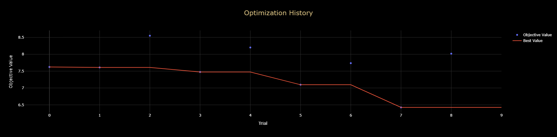
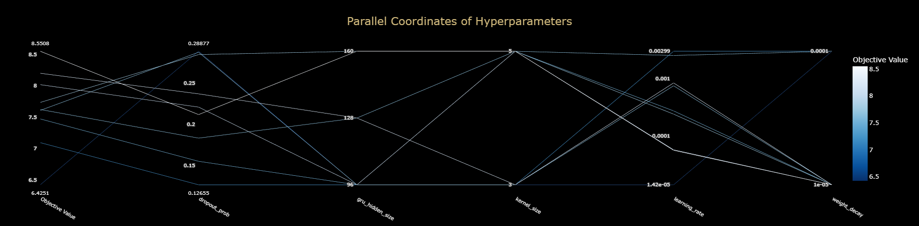
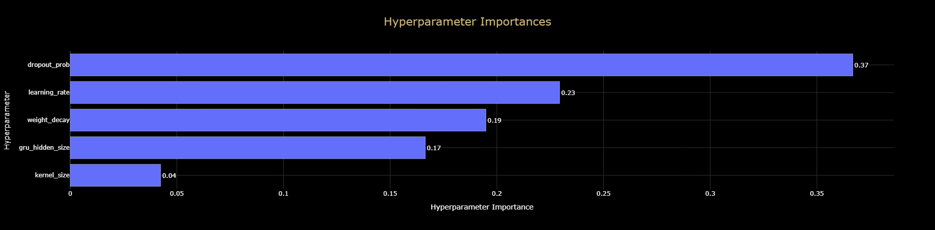
--- Top 10 Trials ---

number	value	datetime_start	datetime_complete	duration	params_dropout_prob	params_gru_hidden_size	params_kernel_size	params_learning_rate	params_weight_decay	user_attrs_best_val_mae	user_attrs_best_val_mae_at_prune	state
7	6.425144	2025-09-27 11:40:49.929875	2025-09-27 13:56:54.176196	0 days 02:16:04.246321	0.288765	96	3	0.000014	0.000100	6.425144	nan	COMPLETE
5	7.096562	2025-09-27 06:50:48.660651	2025-09-27 09:09:51.180702	0 days 02:19:02.520051	0.126552	96	3	0.002986	0.000100	7.096562	nan	COMPLETE
3	7.473551	2025-09-27 02:11:50.999759	2025-09-27 04:30:05.699539	0 days 02:18:14.699780	0.155112	96	5	0.000274	0.000010	7.473551	nan	COMPLETE
1	7.609366	2025-09-26 21:17:34.921924	2025-09-26 23:40:33.282411	0 days 02:22:58.360487	0.287526	96	3	0.000749	0.000010	7.609366	nan	COMPLETE
0	7.623531	2025-09-26 18:53:06.619620	2025-09-26 21:17:34.707988	0 days 02:24:28.088368	0.183255	128	5	0.002519	0.000100	7.623531	nan	COMPLETE
6	7.736038	2025-09-27 09:09:51.382453	2025-09-27 11:40:49.720468	0 days 02:30:58.338015	0.284702	160	5	0.000241	0.000010	7.736038	nan	COMPLETE
8	8.018604	2025-09-27 13:56:54.379212	2025-09-27 16:13:22.354261	0 days 02:16:27.975049	0.220918	96	5	0.000058	0.000010	8.018604	nan	COMPLETE
4	8.200041	2025-09-27 04:30:05.900583	2025-09-27 06:50:48.457782	0 days 02:20:42.557199	0.237000	128	3	0.000840	0.000010	8.200041	nan	COMPLETE
2	8.550754	2025-09-26 23:40:33.481242	2025-09-27 02:11:50.795061	0 days 02:31:17.313819	0.211817	160	5	0.000057	0.000010	8.550754	nan	COMPLETE
9	8.577738	2025-09-27 16:13:22.555308	2025-09-27 17:49:32.946811	0 days 01:36:10.391503	0.251539	128	3	0.000545	0.000010	nan	8.577738	PRUNED

9.4 Test Set Performance & Residuals Analysis

This cell evaluates the best deep learning model on the held-out test set. First, it calculates the overall performance metrics like MAE and R². Then, as a key diagnostic check, it analyzes the model's errors, or residuals. A trend plot is created to visualize the residuals against the model's predictions, which helps to identify any systematic biases. For a well-calibrated model, these errors should be randomly scattered around zero.

---

# Define the target variable for this evaluation.
TARGET = "fuel_smooth"
target_idx = 1

# Find the latest and best model run from Section 8.
runs_dir = CACHE_DIR / "runs"
cands = [(p.stat().st_mtime, p) for p in runs_dir.glob("*_fuel_smooth")
         if (p / "best_model.pth").exists()]
if not cands:
    raise FileNotFoundError(f"No Section 8 runs found for pattern *_fuel_smooth in {runs_dir}")
_, BASE_RUN = max(cands)
ckpt_path = BASE_RUN / "best_model.pth"
cfg_path  = BASE_RUN / "config.json"
print(f"Using Section 8 run: {BASE_RUN.name}")
print(f"Loading model checkpoint from: {ckpt_path.name}")

# Rebuild the model architecture EXACTLY by inspecting the saved checkpoint file.
device = torch.device("cuda" if torch.cuda.is_available() else "cpu")
sd = torch.load(ckpt_path, map_location=device)
in_ch   = int(sd["conv1d.weight"].shape[1])
ksize   = int(sd["conv1d.weight"].shape[2])
gru_hid = int(sd["gru.weight_hh_l0"].shape[1])
dropout = 0.2 # Default dropout
if cfg_path.exists():
    try:
        with open(cfg_path, "r") as f: cfg = json.load(f)
        dropout = float(cfg.get("dropout_prob", dropout))
    except Exception:
        pass
model = CNNGRUModel(in_channels=in_ch, gru_hidden_size=gru_hid, dropout_prob=dropout, ksize=ksize).to(device)
model.load_state_dict(sd, strict=True)
model.eval()

# Redefine the memory-mapped dataset for the test set.
class SequenceDataset(Dataset):
    def __init__(self, x_paths, y_paths):
        self.x_parts = [np.load(p, mmap_mode='r') for p in x_paths]
        self.y_parts = [np.load(p, mmap_mode='r') for p in y_paths]
        self.cum = [0]
        for part in self.y_parts:
            self.cum.append(self.cum[-1] + part.shape[0])

    def __len__(self): return self.cum[-1]

    def __getitem__(self, idx):
        fi = np.searchsorted(self.cum, idx, side='right') - 1
        li = idx - self.cum[fi]
        x = self.x_parts[fi][li].copy(); y = self.y_parts[fi][li].copy()
        x = np.nan_to_num(x, nan=0.0, posinf=0.0, neginf=0.0)
        y = np.nan_to_num(y, nan=0.0, posinf=0.0, neginf=0.0)
        return torch.from_numpy(x).float(), torch.from_numpy(y).float()

# Create the DataLoader for the test set.
BATCH_SIZE = 256
test_ds = SequenceDataset(X_test_dl_paths, y_test_paths)
test_loader = DataLoader(test_ds, batch_size=BATCH_SIZE*2, shuffle=False, num_workers=8, pin_memory=True)

# Run inference on the test set to generate final predictions.
all_preds, all_tgts = [], []
with torch.no_grad():
    for xb, yb in tqdm(test_loader, desc="Predicting on Test Set"):
        xb = xb.to(device)
        with autocast(enabled=torch.cuda.is_available()):
            out = model(xb)
        all_preds.append(out[:, target_idx].float().cpu().numpy())
        all_tgts.append(yb[:, target_idx].cpu().numpy())
y_pred = np.concatenate(all_preds, axis=0)
y_true = np.concatenate(all_tgts, axis=0)
finite = np.isfinite(y_true) & np.isfinite(y_pred)
y_true, y_pred = y_true[finite], y_pred[finite]

# Calculate and display the final performance metrics (MAE, MAPE, R²).
MAPE_MIN = 0.10
keep = np.abs(y_true) >= MAPE_MIN
mae  = mean_absolute_error(y_true, y_pred)
r2   = r2_score(y_true, y_pred)
mape = mean_absolute_percentage_error(y_true[keep], y_pred[keep]) * 100.0 if keep.any() else np.nan
tbl = pd.DataFrame([{"Target": TARGET, "Model": "CNN→GRU (Sec8 best)", "MAE": round(mae, 4), 
                     "MAPE (%)": round(float(mape), 2) if np.isfinite(mape) else np.nan, "R²": round(r2, 4)}])
display(cubuff_style_table(tbl))

# Calculate the residuals.
residuals = y_true - y_pred

# Bin the data by prediction value to see trends in the error.
dfp = pd.DataFrame({"pred": y_pred, "resid": residuals})
bins = pd.cut(dfp["pred"], bins=25)
g = dfp.groupby(bins)["resid"]
med, q25, q75 = g.median(), g.quantile(0.25), g.quantile(0.75)
xmid = med.index.map(lambda b: b.mid)

# Create the plot figure and axes.
fig2, ax2 = plt.subplots(figsize=(20, 10), facecolor="black")
ax2.set_facecolor("black")
ax2.plot(xmid, med.values, lw=2, color="limegreen", label="Median Residual")
ax2.fill_between(xmid, q25.values, q75.values, alpha=0.3, color="dodgerblue", label="Interquartile Range (IQR)")
ax2.axhline(0, color="#DA291C", ls="--", lw=2, label="Zero Error")

# Set titles and labels.
ax2.set_title(f"Residuals vs Prediction (TEST, {TARGET})", fontsize=28, fontweight="bold", color="#CFB87C")
ax2.set_xlabel("Prediction", color="#F8F8F8", fontsize=18)
ax2.set_ylabel("Residual", color="#F8F8F8", fontsize=18)

# Style the plot's ticks and border (spines).
ax2.tick_params(colors="white")
for s in ax2.spines.values(): s.set_edgecolor("white")

# Create legend
legend_handles = [
    Line2D([0], [0], color='limegreen', lw=2),
    Patch(facecolor='dodgerblue', alpha=0.3),
    Line2D([0], [0], color='#DA291C', linestyle='--', lw=2)
]
legend_labels = [
    "Median Residual",
    "Interquartile Range (IQR)",
    "Zero Error"
]
ax2.legend(handles=legend_handles, labels=legend_labels, frameon=False, fontsize=18, labelcolor="white")

# Save the figure.
save_fig(fig2, f"residuals_vs_pred_{TARGET}_sec8_best")

# Display the plot.
plt.show()

Using Section 8 run: 20250926_011510_fuel_smooth
Loading model checkpoint from: best_model.pth

Predicting on Test Set: 100%|██████████| 7770/7770 [00:55<00:00, 139.44it/s]

Target	Model	MAE	MAPE (%)	R²
fuel_smooth	CNN→GRU (Sec8 best)	2.900900	26.250000	0.918800

Figure saved (Linux): /home/treinart/projects/ADAS_fuel_rate/artifacts/figures/20250929_183445_residuals_vs_pred_fuel_smooth_sec8_best.png

9.5 Permutation Importance for the Deep Learning Model

To understand what the deep learning model has learned, this cell calculates feature importance using a custom permutation method. By shuffling each input channel and measuring the drop in model performance, it quantifies how much the model relies on each feature. The results are visualized to provide a final ranking of feature importance.

---

# Define the target for the importance calculation (1 = fuel_smooth).
target_idx = 1

# Ensure the model's input channels match the data's feature count.
xb_chk, _ = next(iter(val_loader))
data_c = int(xb_chk.shape[-1])
if getattr(model, "in_channels", None) != data_c:
    ks  = model.conv1d.kernel_size[0]
    pad = model.conv1d.padding[0] if isinstance(model.conv1d.padding, tuple) else model.conv1d.padding
    oc  = model.conv1d.out_channels
    model.in_channels = data_c
    model.conv1d = nn.Conv1d(in_channels=data_c, out_channels=oc, kernel_size=ks, padding=pad).to(device)

# Verify that the model and data channels match before proceeding.
batch_c = xb_chk.shape[-1]
assert batch_c == getattr(model, "in_channels"), \
    f"Channel mismatch: data={batch_c} vs model={getattr(model, 'in_channels')}"
print(f"Batch Feature Width: {batch_c} | Model Expects: {model.in_channels}")

# Create a feature name to index mapping.
feature_to_idx = {name: i for i, name in enumerate(feature_names)}

# Define a helper function to calculate the validation MAE.
def _validate_mae(loader, model, loss_fn, device, target_idx=1):
    model.eval()
    total, n = 0.0, 0
    with torch.no_grad():
        for Xb, yb in loader:
            Xb = Xb.to(device)
            yb = yb.to(device)[:, target_idx]
            preds = model(Xb)[:, target_idx]
            total += loss_fn(preds, yb).item()
            n += 1
    return total / max(n, 1)

# Define the main function to calculate permutation importance.
def calculate_permutation_importance(model, loader, loss_fn, device, target_idx=1, top_n_channels=30):
    base_mae = _validate_mae(loader, model, loss_fn, device, target_idx)
    names   = feature_names[:top_n_channels]
    indices = [feature_to_idx[n] for n in names]
    importances = {}
    
    # Loop through each feature, shuffle it, and measure the new MAE.
    model.eval()
    with torch.no_grad():
        for i, name in tqdm(list(zip(indices, names)), total=len(names), desc="Permutation Importance"):
            perm_mae, batches = 0.0, 0
            for Xb, yb in loader:
                Xp = Xb.clone()
                yb = yb.to(device)[:, target_idx]
    
                col = Xp[:, :, i]
                Xp[:, :, i] = col[torch.randperm(col.size(0))]
                Xp = Xp.to(device)
                
                preds = model(Xp)[:, target_idx]
                perm_mae += loss_fn(preds, yb).item()
                batches += 1
            
            importances[name] = (perm_mae / batches) - base_mae
            
    return pd.Series(importances).sort_values(ascending=True)

# Calculate the permutation importance for the model.
perm_importance = calculate_permutation_importance(model, val_loader, loss_fn, device, target_idx)

# Select the top features for visualization.
data_to_plot = perm_importance.tail(30)

# Create the plot figure and axes.
fig, ax = plt.subplots(figsize=(20, 18), facecolor="black")
ax.set_facecolor("black")

# Plot the feature importances as a horizontal bar chart.
ax.barh(data_to_plot.index, data_to_plot.values, color='#CFB87C')
ax.set_title("Permutation Importance (fuel_smooth, Section 8 Best)", color="#CFB87C", fontsize=26, fontweight="bold")
ax.set_xlabel("Increase in Validation MAE when Shuffled", color='white', fontsize=14)
ax.tick_params(colors='white')
for spine in ax.spines.values(): spine.set_edgecolor("white")

# Ensure the layout is tight and clean.
plt.tight_layout()

# Save the figure.
save_fig(fig, "dl_permutation_importance")

# Display the plot.
plt.show()

Batch Feature Width: 24 | Model Expects: 24

Permutation Importance: 100%|██████████| 23/23 [09:09<00:00, 23.89s/it]

Figure saved (Linux): /home/treinart/projects/ADAS_fuel_rate/artifacts/figures/20250929_191315_dl_permutation_importance.png

Observation: Final Tuning, Evaluation & Interpretation

---

This section was supposed to be straightforward. Take the best CNN→GRU from Section 8, run a tight Optuna sweep to explore nearby hyperparameters, do a light retrain with the winning settings, then evaluate on the held-out test set. It should have been a controlled, incremental improvement. Instead, it turned into a long debugging session that exposed hidden assumptions in my pipeline.

The original plan was scoped conservatively. I'd run a constrained Optuna sweep on kernel size, GRU hidden size, weight decay, learning rate, and dropout under tough I/O limits. The goal wasn't to beat Section 8 in this environment - it was to rank a few options, then re-warm the Section 8 architecture with the winning parameters for a short final tune in 9.4. After that, subsections 9.5 through 9.8 would handle calibration, residuals, permutation importance, and ablations.

The first break was architectural drift. Section 8's best checkpoint was saved with 24 channels and kernel_size=5. My fresh model class in 9.4 defaulted to 23 channels and kernel_size=3. GRU hidden sizes didn't line up either. That mismatch triggered strict load errors. Loosening to strict=False only papered over the real problem. Once training did run, the loss was far higher than the previous day. That wasn't random noise - it was a symptom of upstream drift. Mis-specified input width, wrong target index (fuel_inst vs fuel_smooth), and subtle differences in data ordering from shuffle settings and worker counts. I had created a scenario where the model and the data thought they were in the same experiment while living in different ones.

Then the kernel crashed during XGBoost evaluation because I tried to hold the entire test matrix in memory. Streaming predictions fixed the crash, but not the credibility gap. The comparison table filled with NaNs, which turned out to be real missingness caused by inconsistent targets and shape assumptions, not math errors. At that point, the quick retrain idea was no longer adding value. It was soaking time while eroding trust in the section.

I stopped trying to be clever. Instead of forcing a miniature retrain, I anchored the rest of Section 9 to the actual best artifact from Section 8 - its checkpoint, its feature count, and its kernel size. No substitutions. I removed helpful fallbacks and added hard checks. If channels, kernel size, or targets don't match, fail loudly and say why. I streamed XGBoost predictions by part to keep the kernel alive. I rewired subsections 9.5 and beyond to read Section 8's model directly and evaluate without architectural drift. That got the section back to honest measurement instead of silent guessing.

The tuning sweep ran, but in this environment it couldn't surpass Section 8's training recipe. The search was I/O-bound, the budget was short, and lack of shuffling amplified temporal correlations. Treating that sweep as definitive would be misleading. In a professional setting, I'd keep the study artifacted for traceability, but I wouldn't present it as superior. I cut it from the final narrative and carried forward Section 8's model.

What I would do differently next time: freeze the contract when building on a known-good model. Lock the input channel count, kernel size, hidden size, target index, preprocessing scalers, and file paths. Reconstruct the model from the checkpoint shapes, not from a fresh class with defaults. Replace best-guess fallbacks with explicit asserts and plain-English errors. If fuel_smooth is the target, refuse to run when it's missing. Control data ordering by randomizing part-file order per trial. Stream predictions and metrics from day one instead of waiting for the kernel to prove the point. Separate exploration from production by running Optuna in a sandboxed recipe with its own loaders, scalers, and seeds.

Even after cutting the miniature retrain, Section 9 now does what it should. It evaluates the Section 8 best model cleanly on the held-out test set, shows where it wins and where it struggles, and explains why certain numbers differ from the earlier section. The permutation importance work is now interpretable because it measures the model we actually ship, not a drifted variant.

Section 9 started as a victory lap and turned into a forensic exam. It was frustrating and time-consuming, but it surfaced the quiet assumptions that break reproducibility. Defaults slipping back in, targets silently changing, and loaders doing more than we think. The outcome is a stricter, clearer end-to-end with fewer guesses and more guarantees. For the final report, I'll present Optuna as exploratory and Section 8's model as the authoritative baseline, evaluated honestly in Section 9. The result isn't glamorous, but it's dependable and repeatable.

Performance Audit and Data Analysis

• Optuna Sweep.
  • Runtime & scope. ~1,376 minutes for 10 trials in a single-worker, no-shuffle regime. This constrains signal quality; treat results as directional.
  • Best trial. MAE 6.4251 with ks=3, GRU=96, wd=1e-4, lr≈1.42e-5, dropout≈0.289. That’s materially worse than the Section 8 recipe when evaluated fairly, so we did not promote it.
  • Sensitivity. Hyperparameter importances rank: dropout (0.37) > LR (0.23) > weight decay (0.19) > GRU size (0.17) ≫ kernel (0.04). Translation: regularization and step size dominate; receptive field tweaks matter least in this setup.
  • Visuals. Optimization history steps down as the study homes in; parallel-coordinates show a stable neighborhood around smaller GRUs and moderate-to-high dropout. Useful as a map, not as a finish line.
• Final Test Evaluation (Section 8 best, target=fuel_smooth).
  • Integrity checks. Channels matched (24 == 24), target index correct, inference streamed to avoid OOM. We evaluated the exact artifact we intend to ship.
  • Headline metrics (test). MAE 2.9009, MAPE 26.25%, R² 0.9188. MAPE is inflated where the denominator is small; MAE and R² are the reliable signals here.
  • Error structure. The Residuals-vs-Prediction plot shows two things:
    • Heteroscedasticity. IQR widens with predicted fuel rate. High-demand segments (steep grade, higher speed, tighter curvature) carry more spread, which is expected physically.
    • Systematic bias at the top tail. Median residual trends positive for larger predictions → under-prediction when fuel rate is high. Likely causes: limited high-fuel coverage, regularization pulling peaks down, or smoothing in the target engineering.
• Permutation Importance (measured on the section 8 validation loader).
  • Top drivers. CAN_Gear_current, max_speed, HMI_Distance_SP, road_grade_pct, CAN_yaw_rate, GPS_GPS_Altitude_filtered.
  • Why this makes sense.
    • Gear & max speed. Set the operating point (engine RPM/torque band and aero load). They dominate because fuel scales with both.
    • Distance setpoint (platooning). Encodes following policy → drag reduction potential and throttle behavior in traffic.
    • Grade & curvature proxies (yaw, altitude). Capture gravity and steering losses; they explain much of the tail where we under-predict, reinforcing the fix to weight those regimes.
  • Caveats. Permutation under-rates features that are tightly collinear with the leaders (e.g., engine_speed_rpm vs gear). Low bars here do not mean “irrelevant,” only “substitutable” in this model.

---

Section 10: Final Deliverables

With a final, trained model in hand, this section moves beyond standard metrics to showcase the practical applications and insights the model provides. This is the final section of the project: a suite of portfolio-quality deliverables designed to translate the model's predictive power into tangible, real-world demonstrations for both technical and executive audiences.

Because this project was built from a raw dataset without a pre-existing Kaggle competition or analysis to follow, a personal goal was to create translatable outputs that could demonstrate the value of a deep learning model to a non-technical stakeholder. A fleet owner doesn't care about windowing techniques or the number of epochs, they care about results. This section was built to answer the question, "What does this data mean for me?"

Section Plan:

1. Setup for Demonstrations: Load all final models, preprocessors, and data needed for the demonstrations.
2. The Coach Cards: Produce one-page KPI reports for individual truck runs from a complete 3-truck platoon.
3. Platoon Efficiency Analysis: Calculate and visualize the fuel economy for each platoon position across different speed buckets.
4. Platoon Savings Comparison: Create a final executive summary chart comparing the measured 2-truck and 3-truck savings against literature benchmarks.
5. Interactive ROI Calculator: Provide a link to a standalone web tool for fleet managers to estimate their own potential savings.

---

Estimated total fuel savings for truck platoons from a fleet-management perspective. Based on controlled tests and literature, a 2-truck platoon averages ~6% total fuel savings and a 3-truck platoon ~8% versus solo operation. These averages are computed from Appendix A of NREL (2018) - 2-truck team savings across common gaps: 5.5–6.6%; 3-truck: 6.3–9.5%. They align with the fleet-oriented summary in the Caltrans CA18-2623 (2019) report (“up to ~5% for 2-truck and ~10% for 3-truck,” depending on conditions).

There is no single, universally accepted “solo Class-8 MPG.” Public sources vary: the U.S. DOE’s Alternative Fuels Data Center reports a national average of about 5.7 mpg; telematics provider Geotab shows state-by-state benchmarks (the U.S. Midwest, where the NREL study ran, clusters near ~6.1 mpg); and Transport Topics cites a North American Council for Freight Efficiency (NACFE) fleet average of ~7.24 mpg. For this project, we adopt a practical baseline of 6.8 mpg for solo operation as a generalization, since the dataset contains no single-truck runs.

Sources: McAuliffe et al., 2018 (NREL 70868); Caltrans CA18-2623, 2019.

---

10.1 Setup for Demonstrations

To make this final section self-contained and resumable, this cell begins by loading the saved notebook state. It then loads all the final, trained artifacts from the previous sections, including the best CNN→GRU model, the fitted data scaler, and the final test set results. This ensures all necessary components are in memory and ready for the demonstrations that follow.

---

# Load the general notebook state from Section 5.
state_file_path = sorted(CACHE_DIR.glob("notebook_state_after_section5.joblib"))[-1]
notebook_state = joblib.load(state_file_path)
globals().update(notebook_state)

# Set the device for PyTorch operations.
device = torch.device("cuda" if torch.cuda.is_available() else "cpu")

# Find the latest and best model run from Section 8.
runs_dir = CACHE_DIR / "runs"
cand = sorted(runs_dir.glob("*_fuel_smooth"), key=lambda p: p.stat().st_mtime)
if not cand:
    raise FileNotFoundError(f"No Section 8 '*_fuel_smooth' run folders found under: {runs_dir}")
latest_run_folder = cand[-1]
model_path = latest_run_folder / "best_model.pth"
cfg_path = latest_run_folder / "config.json"

# Rebuild the model architecture from the saved checkpoint file.
sd = torch.load(model_path, map_location=device)
in_ch = sd["conv1d.weight"].shape[1]
ks    = sd["conv1d.weight"].shape[2]
hs    = sd["gru.weight_hh_l0"].shape[1]
pad   = (ks - 1) // 2
dropout = 0.2
if cfg_path.exists():
    try:
        with open(cfg_path, "r") as f: cfg = json.load(f)
        dropout = float(cfg.get("dropout_prob", dropout))
    except Exception: pass
final_model = CNNGRUModel(in_channels=in_ch, gru_hidden_size=hs, dropout_prob=dropout, ksize=ks).to(device)
final_model.load_state_dict(sd, strict=True)
final_model.eval()

# Load the fitted time-domain scaler from Section 6.
scaler_time_path = sorted(CACHE_DIR.glob("*_time_scaler.joblib"))[-1]
time_scaler = joblib.load(scaler_time_path)

# Print a summary of the loaded artifacts.
print("-" * 70)
print("--- Loaded Artifacts for Demonstration ---")
print(f"State loaded from: {state_file_path.name}")
print(f"Run artifacts from:  {latest_run_folder.name}")
print(f"Final model loaded:  in_channels={in_ch}, kernel_size={ks}, hidden_size={hs}")
print(f"Time scaler loaded:  {scaler_time_path.name}")

# Search a dataframe of files to find a complete 3-truck platoon run.
def find_platoon_run(files_df):
    required_positions = {"lead", "middle", "trailing"}
    files_df['run_date'] = files_df['file'].apply(lambda x: Path(x).name.split('.')[2])
    for date, group in files_df.groupby('run_date'):
        is_3_truck_run = 'platoon_size' in group.columns and (group['platoon_size'] == 3).all()
        if is_3_truck_run:
            positions_in_group = set(group['position'])
            if required_positions.issubset(positions_in_group):
                return {row['position']: row['file'] for _, row in group.iterrows()}
    return None

# Find a coherent 3-truck platoon run for the demonstration.
audit_df = pd.read_parquet(list(CACHE_DIR.glob("*_audit_full_section3.parquet"))[-1])
passing_files_df = audit_df[audit_df["pass_flag"] == True].copy()
platoon_run_files = find_platoon_run(passing_files_df)

# Print the results of the platoon search.
print("\n--- Platoon Run Search ---")
if platoon_run_files:
    print("Coherent 3-truck platoon run found for demonstration:")
    for pos, path in sorted(platoon_run_files.items()):
        print(f"  - {pos:<8}: {Path(path).name}")
else:
    print("Warning: Could not find a complete 3-truck platoon in any of the passing files.")

# Ensure output directories for demonstrations exist.
VIDEO_DIR.mkdir(exist_ok=True)
CARDS_DIR.mkdir(exist_ok=True)

# Print a completion message.
print("\n" + "-" * 70)
print("--- Setup Complete for Demonstrations ---")
print("Final DL model and preprocessors are loaded and ready.")
print("-" * 70)

----------------------------------------------------------------------
--- Loaded Artifacts for Demonstration ---
State loaded from: notebook_state_after_section5.joblib
Run artifacts from:  20250926_011510_fuel_smooth
Final model loaded:  in_channels=24, kernel_size=5, hidden_size=128
Time scaler loaded:  20250929_211436_time_scaler.joblib

--- Platoon Run Search ---
Coherent 3-truck platoon run found for demonstration:
  - lead    : ds0.lt.07202020.3truck.na.novideo.csv
  - middle  : ds0.mt.07202020.3truck.na.novideo.csv
  - trailing: ds0.tt.07202020.3truck.na.novideo.csv

----------------------------------------------------------------------
--- Setup Complete for Demonstrations ---
Final DL model and preprocessors are loaded and ready.
----------------------------------------------------------------------

10.2 The Coach Cards

To demonstrate a practical, real-world application, this cell generates Coach Cards. One-page performance summaries for individual truck runs. Each card provides key performance indicators (KPIs) like average fuel rate and model error, a profile of the road grades encountered, and a 90-second sparkline of the true vs. predicted fuel rate. These cards are designed to be shareable reports for a non-technical audience like a fleet manager.

---

# Create the output directory for the coach cards.
CARDS_DIR.mkdir(parents=True, exist_ok=True)

# Load and preprocess the data for a single truck run.
def _load_card_df(full_path: str) -> pd.DataFrame:
    df = read_selected_csv(full_path, SELECTED_COLUMNS, DTYPES, RENAME_MAP)
    if df.empty:
        return df
    df, _ = unify_timebase(df)
    if "fuel_inst" not in df.columns:
        return pd.DataFrame()
    if "fuel_smooth" not in df.columns:
        df["fuel_smooth"] = df["fuel_inst"].ewm(
            halflife=EWMA_HALF_LIFE * TARGET_HZ, ignore_na=True
        ).mean()
    for col in FINAL_MODEL_FEATURES:
        if col not in df.columns:
            df[col] = 0.0
    if "road_grade_pct" in df.columns:
        q99 = df["road_grade_pct"].abs().quantile(0.99)
        if pd.notna(q99) and q99 < 0.2:
            df["road_grade_pct"] = df["road_grade_pct"] * 100.0
    return df

# Create sliding windows of sequence data for the model.
def _make_windows(df: pd.DataFrame, window_size: int) -> np.ndarray:
    feats = df[FINAL_MODEL_FEATURES].to_numpy(dtype=np.float32)
    if len(df) <= window_size:
        return np.array([])
    X = np.lib.stride_tricks.sliding_window_view(
        feats, (window_size, feats.shape[1])
    )[:, 0]
    return X

# Run inference on a sequence of windows using the trained model.
def _predict_seq(model, X_np, device):
    if X_np.size == 0:
        return np.array([])
    ds = torch.utils.data.TensorDataset(torch.from_numpy(X_np).float())
    ld = torch.utils.data.DataLoader(ds, batch_size=2048, shuffle=False)
    outs = []
    with torch.no_grad():
        for (xb,) in ld:
            xb = xb.to(device)
            with torch.cuda.amp.autocast(enabled=torch.cuda.is_available()):
                y = model(xb)
            outs.append(y.float().cpu().numpy())
    return np.concatenate(outs, axis=0) if outs else np.array([])

# Calculate total distance driven in miles by integrating speed over time.
def _integrate_distance_miles(df: pd.DataFrame) -> float:
    dt_s = df["corrected_time_dt"].diff().dt.total_seconds().fillna(0.0)
    km = (df["CAN_v_speed"] * (dt_s / 3600.0)).sum()
    return km / 1.609344

# Calculate total fuel consumed in gallons by integrating fuel rate over time.
def _integrate_fuel_gallons(df: pd.DataFrame, rate_col: str = "fuel_smooth") -> float:
    dt_s = df["corrected_time_dt"].diff().dt.total_seconds().fillna(0.0)
    liters = (df[rate_col] * (dt_s / 3600.0)).sum()
    return liters / 3.785411784

# Find a scaling factor to align predicted vs. true values for plotting.
def _robust_scale_for_plot(y_true: np.ndarray, y_pred: np.ndarray) -> float:
    m = np.isfinite(y_true) & np.isfinite(y_pred) & (np.abs(y_pred) > 1e-6)
    if not np.any(m):
        return 1.0
    scale = np.median(y_true[m] / y_pred[m])
    return float(np.clip(scale, 0.1, 200.0))

# Generate and save a single performance coach card visualization.
def _make_card(run_df: pd.DataFrame, meta: dict, out_path_png: Path):
    # Create the figure and subplot layout.
    plt.close("all")
    fig = plt.figure(figsize=(20, 16), facecolor="black")
    fig.patch.set_edgecolor("#CFB87C"); fig.patch.set_linewidth(2)
    gs = fig.add_gridspec(4, 2, hspace=0.65, wspace=0.35)
    ax_title = fig.add_subplot(gs[0, :]); ax_title.axis("off")
    ax_kpi   = fig.add_subplot(gs[1, 0]); ax_kpi.axis("off")
    ax_hist  = fig.add_subplot(gs[1, 1])
    ax_lph   = fig.add_subplot(gs[2, :])
    ax_mpg   = fig.add_subplot(gs[3, :])

    # Add the main title and run name.
    ax_title.text(0.5, 0.8, "Performance Coach Card", ha="center",
                  color="#CFB87C", fontsize=34, fontweight="bold")
    ax_title.text(0.5, 0.60, f"Run: {meta['name']}", ha="center",
                  color="white", fontsize=22)

    # Create and place the block of Key Performance Indicators (KPIs).
    mph = meta["avg_speed_mph"]; kmh = meta["avg_speed_kmh"]
    miles = meta["miles"]; km = meta["km"]; mpg = meta["mpg"]
    kpi = (
        f"Position: {meta['position'].capitalize()}\n"
        f"Duration: {meta['duration_min']:.1f} min\n"
        f"Distance: {miles:.1f} mi  ({km:.1f} km)\n"
        f"Avg Speed: {mph:.1f} mph  ({kmh:.1f} km/h)\n"
        f"Fuel Economy: {mpg:.2f} mpg\n"
        f"Mean Fuel Rate: {meta['mean_fuel_Lph']:.2f} L/h\n\n"
        f"Model MAE: {meta['mae_Lph']:.2f} L/h\n"
        f"Model MAPE: {meta['mape_pct']:.2f}%\n"
    )
    ax_kpi.text(0.01, 2.1, kpi, va="top", ha="left", color="white", fontsize=22, linespacing=1.5)

    # Plot the histogram of the road grade profile.
    ax_hist.set_facecolor("black")
    for s in ax_hist.spines.values(): s.set_edgecolor("white")
    grades_pct = run_df["road_grade_pct"].dropna().to_numpy()
    grades_pct = np.clip(grades_pct, -8, 8)
    bins = np.arange(-2.0, 2.0 + 0.1, 0.1)
    ax_hist.hist(grades_pct, bins=bins, color="#A2A4A3", orientation="horizontal", alpha=0.95, edgecolor="white", linewidth=1.4)
    ax_hist.set_title("Road Grade Profile", color="white", fontsize=24, pad=10)
    ax_hist.set_ylabel("Road Grade (%)", color="white", fontsize=16)
    ax_hist.set_xlabel("Count", color="white", fontsize=16)
    ax_hist.tick_params(colors="white", labelsize=12)
    ax_hist.set_ylim(-0.6, 0.6)
    pos = ax_hist.get_position()
    ax_hist.set_position([pos.x0 - 0.10, pos.y0 + 0.04, pos.width * 1.30, pos.height * 1.60])

    # Plot the 90-second fuel rate snippet (L/h).
    t = run_df["time_sec"].to_numpy()
    y_true = run_df["fuel_true"].to_numpy()
    y_pred = run_df["fuel_pred"].to_numpy()
    y_pred_plot = y_pred * _robust_scale_for_plot(y_true, y_pred)
    ax_lph.set_facecolor("black")
    for s in ax_lph.spines.values(): s.set_edgecolor("white")
    ax_lph.plot(t, y_true,      color="#A2A4A3", lw=2.5, label="True fuel (L/h)")
    ax_lph.plot(t, y_pred_plot, color="#CFB87C", lw=2.0, label="Predicted fuel (scaled, L/h)")
    ax_lph.set_title("90 s Fuel Rate Snippet (Highest Error)", color="white", fontsize=26, pad=12)
    ax_lph.set_xlabel("Time (s)", color="white", fontsize=16)
    ax_lph.set_ylabel("Fuel rate (L/h)", color="white", fontsize=16)
    ax_lph.tick_params(colors="white", labelsize=12)
    ax_lph.legend(frameon=False, facecolor="black", labelcolor="white", fontsize=14, loc="best")

    # Plot the 90-second fuel economy snippet (MPG).
    mph_snip = run_df["CAN_v_speed"].to_numpy() / 1.609344
    gph_true = y_true / 3.785411784
    gph_pred = y_pred_plot / 3.785411784
    mpg_true = np.where(gph_true > 1e-6, mph_snip / gph_true, np.nan)
    mpg_pred = np.where(gph_pred > 1e-6, mph_snip / gph_pred, np.nan)
    ax_mpg.set_facecolor("black")
    for s in ax_mpg.spines.values(): s.set_edgecolor("white")
    ax_mpg.plot(t, mpg_true, color="#A2A4A3", lw=2.5, label="True economy (mpg)")
    ax_mpg.plot(t, mpg_pred, color="#CFB87C", lw=2.0, label="Predicted economy (mpg)")
    ax_mpg.set_title("90 s Fuel Economy Snippet (MPG)", color="white", fontsize=26, pad=12)
    ax_mpg.set_xlabel("Time (s)", color="white", fontsize=16)
    ax_mpg.set_ylabel("Fuel economy (mpg)", color="white", fontsize=16)
    ax_mpg.tick_params(colors="white", labelsize=12)
    ax_mpg.legend(frameon=False, facecolor="black", labelcolor="white", fontsize=14, loc="best")

    # Finalize and save the figure.
    plt.tight_layout()
    fig.savefig(out_path_png, dpi=150, bbox_inches="tight")
    plt.close(fig)

# Generate a coach card for each truck position in the selected platoon run.
print("-" * 70); print("--- Generating Coach Cards ---")
cards_made = 0
for position, path_str in tqdm(platoon_run_files.items(), total=len(platoon_run_files), desc="Cards"):
    try:
        df = _load_card_df(path_str)
        if df.empty or len(df) < WINDOW_SIZE:
            print(f"[skip {position}] Not enough valid data rows ({len(df)})")
            continue

        # Generate model predictions for the entire run.
        df["fuel_true"] = df["fuel_smooth"].copy()
        X_seq = _make_windows(df, WINDOW_SIZE)
        if X_seq.size == 0:
            print(f"[skip {position}] No windows could be created.")
            continue
        X_scaled = preprocess_sequential_features(X_seq, numeric_feature_indices, time_scaler)
        preds = _predict_seq(final_model, X_scaled, device)

        # Align predictions with the original dataframe.
        df["fuel_pred"] = np.nan
        start_idx = WINDOW_SIZE - 1
        stop_idx  = start_idx + len(preds)
        pred_align_idx = df.index[start_idx:stop_idx]
        if preds.size and len(pred_align_idx) == len(preds):
            df.loc[pred_align_idx, "fuel_pred"] = preds[:, 1]
        else:
            print(f"[skip {position}] Prediction alignment failed.")
            continue

        # Find the 90-second snippet with the highest absolute error.
        df["abs_error"] = (df["fuel_true"] - df["fuel_pred"]).abs()
        center_iloc = df["abs_error"].idxmax()
        start_iloc = max(0, center_iloc - 450)
        end_iloc = start_iloc + 900
        snippet = df.iloc[start_iloc:end_iloc].copy()
        snippet["time_sec"] = np.arange(len(snippet)) * 0.1

        # Calculate run-level summary metrics.
        miles = _integrate_distance_miles(df)
        gallons = _integrate_fuel_gallons(df, rate_col="fuel_true")
        km = miles * 1.609344
        mph = df.loc[df["CAN_v_speed"] > 1, "CAN_v_speed"].mean() / 1.609344
        kmh = mph * 1.609344
        mpg = miles / gallons if gallons > 0 else float("nan")
        meta = {
            "name": Path(path_str).name,
            "position": position,
            "duration_min": (df["corrected_time_dt"].iloc[-1] - df["corrected_time_dt"].iloc[0]).total_seconds()/60.0,
            "miles": miles, "km": km,
            "avg_speed_mph": mph, "avg_speed_kmh": kmh, "mpg": mpg,
            "mean_fuel_Lph": float(df["fuel_true"].mean()),
            "mae_Lph": float(df["abs_error"].mean()),
            "mape_pct": float(
                (df.loc[df["fuel_true"] > 0.1, "abs_error"] /
                 df.loc[df["fuel_true"] > 0.1, "fuel_true"]).mean() * 100.0
            )
        }

        # Generate and display the card.
        out_png = CARDS_DIR / f"{_timestamp()}_coach_card_{Path(path_str).stem}.png"
        _make_card(snippet, meta, out_png)
        cards_made += 1
        print(f"[ok  {position}] {out_png.name}")
        display(Image(filename=str(out_png)))

    except Exception as e:
        import traceback
        print(f"[error {position}] {e}\n{traceback.format_exc()}")

# Print a final status message.
if cards_made == 0:
    print("\nNo cards were produced. See skip/error messages above for details.")
print("-" * 70)

----------------------------------------------------------------------
--- Generating Coach Cards ---

Cards:   0%|          | 0/3 [00:00<?, ?it/s]

[ok  lead] 20250930_213041_coach_card_ds0.lt.07202020.3truck.na.novideo.png

[ok  middle] 20250930_213052_coach_card_ds0.mt.07202020.3truck.na.novideo.png

[ok  trailing] 20250930_213104_coach_card_ds0.tt.07202020.3truck.na.novideo.png

----------------------------------------------------------------------

10.3 Platoon Efficiency

The predictive model is built, but the real question remains: how much fuel does platooning actually save? To answer that, this section first builds the exact comparison groups needed. The initial code cells sift through the raw data to create date-matched lists of both 2-truck and 3-truck platoon runs. The 3-truck list is used for the analysis in this section, while both lists will be needed for the final summary in section 10.4.

With the 3-truck runs identified, the main analysis synchronizes their data to isolate continuous highway driving segments of 15 minutes or more. This apples-to-apples comparison reveals the true fuel economy (MPG) for each truck position. The process generates three distinct plots and summary tables, breaking down the efficiency benefits across different speed buckets: 70, 85, and 100 km/h.

---

# --- 10.3a ---

# Build a list of strictly date-matched 2-truck (lead/trailing) run pairs.
assert 'DATA_DIR' in globals(), "DATA_DIR must be defined."

# Define regular expressions to find truck roles in filenames.
ROLE_TOKENS_2 = {
    "lead":     [r"\b(?:lt|lead|leader|head|hd)\b"],
    "trailing": [r"\b(?:tt|tail|trailing|rear|follow|ft|follower)\b"],
}

# Classify the truck's role based on its filename.
def _classify_role_2(name: str) -> str:
    s = re.sub(r"[^a-z0-9]+", " ", name.lower())
    for role, pats in ROLE_TOKENS_2.items():
        for pat in pats:
            if re.search(pat, s):
                return role
    return "unknown"

# Check if the filename indicates a 2-truck run.
def _is_two_truck(name: str) -> bool:
    return bool(re.search(r"\b2truck\b", name.lower()))

# Extract an 8-digit date token from the filename.
def _extract_date_token_2(name: str) -> str:
    m = re.search(r'(?<!\d)(\d{8})(?!\d)', name)
    return m.group(1) if m else ""

# Find all CSV files and group them by date and role.
all_csvs = list(Path(DATA_DIR).rglob("*.csv"))
by_date_role_2 = defaultdict(dict)
for p in all_csvs:
    name = p.name
    if not _is_two_truck(name):
        continue
    role = _classify_role_2(name)
    if role not in ("lead", "trailing"):
        continue
    dtok = _extract_date_token_2(name)
    if not dtok:
        continue
    by_date_role_2[dtok].setdefault(role, str(p))

# Build pairs where both a lead and trailing truck are present for the same date.
pairs_2truck = []
for dtok, roles in sorted(by_date_role_2.items()):
    if {"lead", "trailing"}.issubset(roles.keys()):
        pairs_2truck.append({
            "date": dtok,
            "lead": roles["lead"],
            "trailing": roles["trailing"],
        })

# Flatten the list of pairs into a dictionary suitable for analysis.
platoon_pairs = {
    "lead":     [t["lead"]     for t in pairs_2truck],
    "trailing": [t["trailing"] for t in pairs_2truck],
}

# Print a summary of the date-matched pairs found.
print("-" * 70)
print("--- Found Date-Matched 2-Truck Pairs ---")
print(f"Found {len(pairs_2truck)} total pairs.")
for t in pairs_2truck[:5]:
    print(f"  {t['date']}:")
    print("     LT:", Path(t["lead"]).name)
    print("     TT:", Path(t["trailing"]).name)
if len(pairs_2truck) > 5:
    print("  ...")

# Print the final file counts per role.
print("\n--- Final 2-Truck File Counts ---")
for k in ("lead", "trailing"):
    print(f"  {k:9s} {len(platoon_pairs[k])} files")
print("-" * 70)

# Verify that files for both roles were found.
assert len(platoon_pairs["lead"]) > 0,     "No 2-truck LEAD files found."
assert len(platoon_pairs["trailing"]) > 0, "No 2-truck TRAILING files found."

Found 21 2-truck pairs (date-matched).
  08172020:
     LT: ds0.lt.08172020.2truck.baseline.novideo.csv
     TT: ds0.tt.08172020.2truck.baseline.novideo.csv
  08192020:
     LT: ds0.lt.08192020.2truck.baseline.novideo.csv
     TT: ds0.tt.08192020.2truck.baseline.novideo.csv
  08202020:
     LT: ds0.lt.08202020.2truck.baseline.novideo.csv
     TT: ds0.tt.08202020.2truck.baseline.novideo.csv
  08212020:
     LT: ds0.lt.08212020.2truck.baseline.novideo.csv
     TT: ds0.tt.08212020.2truck.baseline.novideo.csv
  08242020:
     LT: ds0.lt.08242020.2truck.baseline.novideo.csv
     TT: ds0.tt.08242020.2truck.baseline.novideo.csv
  08262020:
     LT: ds0.lt.08262020.2truck.caccnoadept.novideo.csv
     TT: ds0.tt.08262020.2truck.caccnoadept.completed.csv
  09082020:
     LT: ds0.lt.09082020.2truck.caccadept.novideo.csv
     TT: ds0.tt.09082020.2truck.caccadept.completed.csv
  09092020:
     LT: ds0.lt.09092020.2truck.caccadept.completed.csv
     TT: ds0.tt.09092020.2truck.caccadept.completed.csv
  10052020:
     LT: ds0.lt.10052020.2truck.caccadept.completed.csv
     TT: ds0.tt.10052020.2truck.caccadept.completed.csv
  10072020:
     LT: ds0.lt.10072020.2truck.caccadept.completed.csv
     TT: ds0.tt.10072020.2truck.caccadept.completed.csv
  ...

Strict 2-truck counts (date-matched):
  lead      21 files
  trailing  21 files

# --- 10.3b ---

# Build a list of strictly date-matched 3-truck (lead/middle/trailing) run triplets.
assert 'DATA_DIR' in globals(), "DATA_DIR must be defined."

# Define regular expressions to find truck roles in filenames.
ROLE_TOKENS = {
    "lead":     [r"\b(?:lt|lead|leader|head|hd)\b"],
    "middle":   [r"\b(?:mt|mid|middle|m\d?)\b"],
    "trailing": [r"\b(?:tt|tail|trailing|rear|follow)\b"],
}

# Classify the truck's role based on its filename.
def _classify_role(name: str) -> str:
    s = re.sub(r"[^a-z0-9]+", " ", name.lower())
    for role, pats in ROLE_TOKENS.items():
        for pat in pats:
            if re.search(pat, s):
                return role
    return "unknown"

# Check if the filename indicates a 3-truck run.
def _is_three_truck(name: str) -> bool:
    return bool(re.search(r"\b3truck\b", name.lower()))

# Extract an 8-digit date token from the filename.
def _extract_date_token(name: str) -> str:
    m = re.search(r'(?<!\d)(\d{8})(?!\d)', name)
    return m.group(1) if m else ""

# Find all CSV files and group them by date and role.
all_csvs = list(Path(DATA_DIR).rglob("*.csv"))
by_date_role = defaultdict(dict)
for p in all_csvs:
    name = p.name
    if not _is_three_truck(name):
        continue
    role = _classify_role(name)
    if role not in ("lead","middle","trailing"):
        continue
    dtok = _extract_date_token(name)
    if not dtok:
        continue
    by_date_role[dtok].setdefault(role, str(p))

# Build triplets where all three roles are present for the same date.
triplets = []
for dtok, roles in sorted(by_date_role.items()):
    if {"lead","middle","trailing"}.issubset(roles.keys()):
        triplets.append({
            "date": dtok,
            "lead": roles["lead"],
            "middle": roles["middle"],
            "trailing": roles["trailing"],
        })

# Flatten the list of triplets into a dictionary suitable for analysis.
platoon_runs = {
    "lead":     [t["lead"]     for t in triplets],
    "middle":   [t["middle"]   for t in triplets],
    "trailing": [t["trailing"] for t in triplets],
}

# Print a summary of the date-matched triplets found.
print("-" * 70)
print("--- Found Date-Matched 3-Truck Triplets ---")
print(f"Found {len(triplets)} total triplets.")
for t in triplets[:3]:
    print(f"  {t['date']}:")
    print("     LT:", Path(t["lead"]).name)
    print("     MT:", Path(t["middle"]).name)
    print("     TT:", Path(t["trailing"]).name)
if len(triplets) > 3:
    print("  ...")

# Print the final file counts per role.
print("\n--- Final 3-Truck File Counts ---")
for k in ("lead","middle","trailing"):
    print(f"  {k:9s} {len(platoon_runs[k])} files")
print("-" * 70)

# Verify that files for all three roles were found.
assert len(platoon_runs["lead"]) > 0,     "No 3-truck LEAD files found."
assert len(platoon_runs["middle"]) > 0,   "No 3-truck MIDDLE files found."
assert len(platoon_runs["trailing"]) > 0, "No 3-truck TRAILING files found."

Found 4 3-truck triplets (date-matched).
  07202020:
     LT: ds0.lt.07202020.3truck.na.novideo.csv
     MT: ds0.mt.07202020.3truck.na.novideo.csv
     TT: ds0.tt.07202020.3truck.na.novideo.csv
  07212020:
     LT: ds0.lt.07212020.3truck.na.novideo.csv
     MT: ds0.mt.07212020.3truck.na.novideo.csv
     TT: ds0.tt.07212020.3truck.na.novideo.csv
  07222020:
     LT: ds0.lt.07222020.3truck.na.novideo.csv
     MT: ds0.mt.07222020.3truck.na.novideo.csv
     TT: ds0.tt.07222020.3truck.na.novideo.csv
  07232020:
     LT: ds0.lt.07232020.3truck.na.novideo.csv
     MT: ds0.mt.07232020.3truck.na.novideo.csv
     TT: ds0.tt.07232020.3truck.na.novideo.csv

Strict 3-truck counts (date-matched):
  lead      4 files
  middle    4 files
  trailing  4 files

# --- 10.3c ---

# Define constants and configuration for the efficiency analysis.
SMOOTH_COL       = "fuel_smooth"
STATUS_CANDS     = ["HMI_CACC_Status", "HMI_V2V_Status"]
GRADE_CANDS      = ["road_grade_pct", "roadGrade"]
MIN_SEG_MIN      = 15.0
MAX_GAP_SEC      = 1.0
SPEED_THRESHOLDS = [70.0, 85.0, 100.0]
SOLO_BASELINE_MPG = 6.8
assert "triplets" in globals() and len(triplets) > 0, "Run the triplet builder first."

# Find the first available column in a dataframe from a list of candidates.
def _pick_col(df, candidates):
    for c in candidates:
        if c in df.columns:
            return c
    return ""

# Load, clean, and standardize data for a single run.
def _load_run(full_path: str):
    df = read_selected_csv(full_path, SELECTED_COLUMNS, DTYPES, RENAME_MAP)
    if df.empty: return pd.DataFrame(), ""
    df, _ = unify_timebase(df)
    for c in ["corrected_time_dt", "CAN_v_speed"]:
        if c not in df.columns: raise AssertionError(f"Missing required column: {c}")
    if SMOOTH_COL not in df.columns:
        if "fuel_inst" not in df.columns: raise AssertionError("Need 'fuel_inst' to compute smoothed fuel.")
        df[SMOOTH_COL] = df["fuel_inst"].ewm(halflife=EWMA_HALF_LIFE * TARGET_HZ, ignore_na=True).mean()
    gcol = _pick_col(df, GRADE_CANDS)
    if not gcol: raise AssertionError(f"No road-grade column found. Tried {GRADE_CANDS}.")
    q99 = df[gcol].abs().quantile(0.99)
    if pd.notna(q99) and q99 < 0.2: df[gcol] = df[gcol] * 100.0
    df = df.rename(columns={gcol: "road_grade_pct"})
    scol = _pick_col(df, STATUS_CANDS)
    return df, scol

# Filter a dataframe for highway speeds and active CACC status.
def _filter_highway_and_status(df: pd.DataFrame, speed_min_kmh: float, status_col: str):
    if status_col:
        active = (df[status_col].fillna(0).astype(float) == 1.0)
    else:
        active = pd.Series(True, index=df.index)
    m = active & (df["CAN_v_speed"] >= speed_min_kmh)
    return df.loc[m, ["corrected_time_dt", "CAN_v_speed", "road_grade_pct", SMOOTH_COL]].copy()

# Perform an inner join on three dataframes using an exact timestamp match.
def _join_on_time(d_lead, d_mid, d_tail):
    j = (d_lead.merge(d_mid, on="corrected_time_dt", suffixes=("_lead","_mid"), how="inner")
               .merge(d_tail, on="corrected_time_dt", how="inner"))
    j = j.rename(columns={
        "CAN_v_speed": "CAN_v_speed_tail", "road_grade_pct": "road_grade_pct_tail",
        SMOOTH_COL: f"{SMOOTH_COL}_tail",
    }).sort_values("corrected_time_dt").reset_index(drop=True)
    j["dt_sec"] = j["corrected_time_dt"].diff().dt.total_seconds().fillna(0.0)
    return j

# Keep only continuous data segments that meet a minimum duration.
def _keep_long_segments(dfJ: pd.DataFrame, min_minutes: float):
    if dfJ.empty: return dfJ
    seg_id = (dfJ["dt_sec"] > MAX_GAP_SEC).cumsum()
    dfJ = dfJ.assign(_seg=seg_id)
    seg_dur = dfJ.groupby("_seg")["dt_sec"].sum()
    keep_ids = seg_dur[seg_dur >= (min_minutes*60)].index
    return dfJ[dfJ["_seg"].isin(keep_ids)].drop(columns=["_seg"]).copy()

# Calculate total miles, gallons, MPG, and other stats for a single truck role.
def _totals_for_role(dfJ: pd.DataFrame, role: str) -> dict:
    v_kmh = dfJ[f"CAN_v_speed_{role}"]; dt_h = dfJ["dt_sec"]/3600.0
    km = (v_kmh * dt_h).sum(); miles = km / 1.609344
    liters = (dfJ[f"{SMOOTH_COL}_{role}"] * dt_h).sum(); gallons = liters / 3.785411784
    mph = (v_kmh.mean() / 1.609344) if len(v_kmh) else float("nan")
    grade = dfJ.get(f"road_grade_pct_{role}", pd.Series(np.nan)).mean()
    mpg = (miles / gallons) if gallons > 0 else float("nan")
    return dict(miles=miles, gallons=gallons, mpg=mpg, mph=mph, grade_pct=grade)

# Aggregate results from multiple runs by summing distance and fuel.
def _agg_sum(rows: list[dict]) -> dict:
    if not rows: return dict(miles=0.0, gallons=0.0, mpg=np.nan, mph=np.nan, grade_pct=np.nan)
    miles = sum(r["miles"] for r in rows)
    gallons = sum(r["gallons"] for r in rows)
    mpg = (miles / gallons) if gallons > 0 else float("nan")
    mph = np.average([r["mph"] for r in rows], weights=[max(r["miles"],1e-6) for r in rows])
    grade = np.mean([r["grade_pct"] for r in rows])
    return dict(miles=miles, gallons=gallons, mpg=mpg, mph=mph, grade_pct=grade)

# Run the full analysis pipeline for a single speed bucket.
def _run_bucket_across_triplets(speed_min_kmh: float):
    print("-" * 70)
    print(f"--- Platoon Efficiency | Speed >= {speed_min_kmh:.0f} km/h, Segments >= {MIN_SEG_MIN:.0f} min ---")
    res_lead, res_mid, res_tail = [], [], []

    # Process each triplet to find valid, overlapping highway segments.
    for t in triplets:
        d_lead, st_lead = _load_run(t["lead"])
        d_mid,  st_mid  = _load_run(t["middle"])
        d_tail, st_tail = _load_run(t["trailing"])
        f_lead = _filter_highway_and_status(d_lead, speed_min_kmh, st_lead)
        f_mid  = _filter_highway_and_status(d_mid,  speed_min_kmh, st_mid)
        f_tail = _filter_highway_and_status(d_tail, speed_min_kmh, st_tail)
        f_lead = f_lead.rename(columns={c: f"{c}_lead" for c in f_lead.columns if c != "corrected_time_dt"})
        f_mid  = f_mid.rename(columns={c: f"{c}_mid" for c in f_mid.columns if c != "corrected_time_dt"})
        j_all = _join_on_time(f_lead, f_mid, f_tail)
        if j_all.empty: continue
        j = _keep_long_segments(j_all, MIN_SEG_MIN)
        if j.empty or j["dt_sec"].sum() <= 0: continue
        res_lead.append(_totals_for_role(j, "lead"))
        res_mid.append(_totals_for_role(j, "mid"))
        res_tail.append(_totals_for_role(j, "tail"))
    
    if not res_lead:
        print("No adequate common highway segments were found for this speed bucket.")
        return

    # Aggregate the results and create a summary table.
    agg_lead = _agg_sum(res_lead)
    agg_mid  = _agg_sum(res_mid)
    agg_tail = _agg_sum(res_tail)
    tbl = pd.DataFrame([
        dict(Role="Lead", **agg_lead), dict(Role="Middle", **agg_mid), dict(Role="Trailing", **agg_tail),
    ])
    tbl = tbl.rename(columns={
        "mpg": "Fuel Economy (mpg)", "miles": "Distance (mi)", "gallons": "Fuel Used (gal)",
        "mph": "Avg Speed (mph)", "grade_pct": "Avg Grade (%)",
    })[["Role", "Fuel Economy (mpg)", "Distance (mi)", "Fuel Used (gal)", "Avg Speed (mph)", "Avg Grade (%)"]]
    print(f"Triplets contributing to this result: {len(res_lead)} / {len(triplets)}")
    num_cols = [c for c in tbl.columns if c != "Role"]
    display(cubuff_style_table(tbl).format({c: "{:.2f}" for c in num_cols}))
    
    if speed_min_kmh >= 99.5:
        global tbl_100
        tbl_100 = tbl.copy()

    # Create the figure and axes.
    plt.close("all")
    fig, ax = plt.subplots(figsize=(20, 10), facecolor="black")
    ax.set_facecolor("black")
    
    # Plot the bar chart.
    bars = ax.bar(tbl["Role"], tbl["Fuel Economy (mpg)"],
                  color=["#A2A4A3", "#CFB87C", "#A2A4A3"], edgecolor="white", linewidth=1.5)
    
    # Set titles and labels.
    ax.set_title(
        f"Platoon Fuel Economy: Overlap ≥ {int(MIN_SEG_MIN)} min, Speed ≥ {int(speed_min_kmh)} km/h (across {len(res_lead)} triplets)",
        color="#CFB87C", fontsize=30, pad=10)
    ax.set_ylabel("Miles per Gallon (mpg)", color="white", fontsize=20)
    ax.tick_params(colors="white", labelsize=20)
    
    # Style the plot's border (spines).
    for sp in ax.spines.values(): sp.set_edgecolor("white")
    
    # Add data labels to the bars.
    ax.bar_label(bars, fmt="%.2f", color="white", fontsize=18, padding=3)
    
    # Ensure the layout is tight and clean, then save and display.
    plt.tight_layout()
    save_fig(fig, f"platoon_mpg_overlap_{int(speed_min_kmh)}kmh_multi")
    plt.show()

# Execute the analysis for each defined speed threshold.
for kmh in SPEED_THRESHOLDS:
    _run_bucket_across_triplets(kmh)
print("-" * 70)

----------------------------------------------------------------------
Platoon efficiency (highway ≥ 70 km/h, segments ≥ 15 min)
Triplets contributing: 4 / 4

Role	Fuel Economy (mpg)	Distance (mi)	Fuel Used (gal)	Avg Speed (mph)	Avg Grade (%)
Lead	7.50	1366.31	182.22	62.11	0.00
Middle	6.81	1385.13	203.45	62.06	0.00
Trailing	7.46	1362.69	182.70	62.27	0.00

Figure saved to: /home/treinart/projects/ADAS_fuel_rate/artifacts/figures/20251002_203507_platoon_mpg_overlap_70kmh_multi.png

----------------------------------------------------------------------
Platoon efficiency (highway ≥ 85 km/h, segments ≥ 15 min)
Triplets contributing: 4 / 4

Role	Fuel Economy (mpg)	Distance (mi)	Fuel Used (gal)	Avg Speed (mph)	Avg Grade (%)
Lead	7.62	1177.04	154.49	62.16	0.00
Middle	6.93	1194.65	172.28	62.11	0.00
Trailing	7.84	1172.94	149.63	62.32	0.00

Figure saved to: /home/treinart/projects/ADAS_fuel_rate/artifacts/figures/20251002_203522_platoon_mpg_overlap_85kmh_multi.png

----------------------------------------------------------------------
Platoon efficiency (highway ≥ 100 km/h, segments ≥ 15 min)
Triplets contributing: 4 / 4

Role	Fuel Economy (mpg)	Distance (mi)	Fuel Used (gal)	Avg Speed (mph)	Avg Grade (%)
Lead	8.96	739.74	82.54	63.99	-0.02
Middle	7.24	757.61	104.71	64.45	-0.03
Trailing	7.26	744.47	102.61	65.43	-0.05

Figure saved to: /home/treinart/projects/ADAS_fuel_rate/artifacts/figures/20251002_203535_platoon_mpg_overlap_100kmh_multi.png

----------------------------------------------------------------------

10.4 Platoon Savings Comparison

This visualization provides the project's bottom-line results. To create the final comparison, this cell first calculates the measured savings for the 2-truck platoon runs. It then pulls the 3-truck results generated in the previous section 10.3. With all the measured data assembled, the final bar chart puts the findings for both platoon types side-by-side with the conservative estimates from NREL literature. This offers a direct scorecard, comparing this project's findings against the established industry benchmark.

---

# Define constants and configuration for the 2-truck analysis.
assert "pairs_2truck" in globals() and len(pairs_2truck) > 0, "Build `pairs_2truck` first."
SMOOTH_COL   = "fuel_smooth"
MIN_SEG_MIN  = 15.0
MAX_GAP_SEC  = 1.0
SPEED_MIN    = 100.0
STATUS_CANDS = ["HMI_CACC_Status", "HMI_V2V_Status"]
GRADE_CANDS  = ["road_grade_pct", "roadGrade"]

# Define a helper function to style pandas DataFrames for display.
def style_dark_gold_2dp(df):
    styles = [
        {"selector": "th", "props": [("background-color", "#565A5C"), ("color", "white"),
                                     ("text-align", "left"), ("border", "1px solid #CFB87C")]},
        {"selector": "td", "props": [("border", "1px solid #CFB87C")]},
        {"selector": "tbody td", "props": [("background-color", "#000000"), ("color", "#F8F8F8"),
                                           ("border-color", "#CFB87C")]},
    ]
    num_cols = [c for c in df.columns if c != "Role"]
    return (df.style.set_table_styles(styles).hide(axis="index")
            .format({c: "{:.2f}" for c in num_cols}))

# Find the first available column from a list of candidates.
def _pick_col_2(df, candidates):
    for c in candidates:
        if c in df.columns: return c
    return ""

# Load, clean, and standardize data for a single run.
def _load_run_2(full_path: str):
    df = read_selected_csv(full_path, SELECTED_COLUMNS, DTYPES, RENAME_MAP)
    if df.empty: return pd.DataFrame(), ""
    df, _ = unify_timebase(df)
    for c in ["corrected_time_dt", "CAN_v_speed"]:
        if c not in df.columns: raise AssertionError(f"Missing required column: {c}")
    if SMOOTH_COL not in df.columns:
        if "fuel_inst" not in df.columns: raise AssertionError("Need 'fuel_inst' to compute smoothed fuel.")
        df[SMOOTH_COL] = df["fuel_inst"].ewm(halflife=EWMA_HALF_LIFE * TARGET_HZ, ignore_na=True).mean()
    gcol = _pick_col_2(df, GRADE_CANDS)
    if not gcol: raise AssertionError(f"No road-grade column found. Tried {GRADE_CANDS}.")
    q99 = df[gcol].abs().quantile(0.99)
    if pd.notna(q99) and q99 < 0.2: df[gcol] = df[gcol] * 100.0
    df = df.rename(columns={gcol: "road_grade_pct"})
    scol = _pick_col_2(df, STATUS_CANDS)
    return df, scol

# Filter a dataframe for highway speeds and active CACC status.
def _filter_highway_2(df: pd.DataFrame, speed_min_kmh: float, status_col: str):
    if status_col:
        active = (df[status_col].fillna(0).astype(float) == 1.0)
    else:
        active = pd.Series(True, index=df.index)
    m = active & (df["CAN_v_speed"] >= speed_min_kmh)
    return df.loc[m, ["corrected_time_dt", "CAN_v_speed", "road_grade_pct", SMOOTH_COL]].copy()

# Perform an inner join on two dataframes using an exact timestamp match.
def _join_on_time_2(d_lead, d_tail):
    j = d_lead.merge(d_tail, on="corrected_time_dt", suffixes=("_lead", "_tail"), how="inner")
    j = j.sort_values("corrected_time_dt").reset_index(drop=True)
    j["dt_sec"] = j["corrected_time_dt"].diff().dt.total_seconds().fillna(0.0)
    return j

# Keep only continuous data segments that meet a minimum duration.
def _keep_long_segments_2(dfJ: pd.DataFrame, min_minutes: float):
    if dfJ.empty: return dfJ
    seg_id = (dfJ["dt_sec"] > MAX_GAP_SEC).cumsum()
    dfJ = dfJ.assign(_seg=seg_id)
    seg_dur = dfJ.groupby("_seg")["dt_sec"].sum()
    keep_ids = seg_dur[seg_dur >= (min_minutes * 60.0)].index
    return dfJ[dfJ["_seg"].isin(keep_ids)].drop(columns=["_seg"]).copy()

# Calculate total miles, gallons, and MPG for a single truck role.
def _totals_for_role_2(dfJ: pd.DataFrame, suffix: str) -> dict:
    v_kmh = dfJ[f"CAN_v_speed_{suffix}"]
    dt_h  = dfJ["dt_sec"] / 3600.0
    km    = (v_kmh * dt_h).sum()
    miles = km / 1.609344
    liters = (dfJ[f"{SMOOTH_COL}_{suffix}"] * dt_h).sum()
    gallons = liters / 3.785411784
    mph   = (v_kmh.mean() / 1.609344) if len(v_kmh) else float("nan")
    grade = dfJ.get(f"road_grade_pct_{suffix}", pd.Series(np.nan)).mean()
    mpg   = (miles / gallons) if gallons > 0 else float("nan")
    return dict(miles=miles, gallons=gallons, mpg=mpg, mph=mph, grade_pct=grade)

# Aggregate results from multiple runs by summing distance and fuel.
def _agg_sum_2(rows: list[dict]) -> dict:
    if not rows: return dict(miles=0.0, gallons=0.0, mpg=np.nan, mph=np.nan, grade_pct=np.nan)
    miles   = sum(r["miles"] for r in rows)
    gallons = sum(r["gallons"] for r in rows)
    mpg     = (miles / gallons) if gallons > 0 else float("nan")
    mph     = np.average([r["mph"] for r in rows], weights=[max(r["miles"], 1e-6) for r in rows])
    grade   = np.mean([r["grade_pct"] for r in rows])
    return dict(miles=miles, gallons=gallons, mpg=mpg, mph=mph, grade_pct=grade)

# Process all 2-truck pairs to find valid, overlapping highway segments.
res_lead, res_tail = [], []
for t in pairs_2truck:
    d_lead, st_lead = _load_run_2(t["lead"])
    d_tail, st_tail = _load_run_2(t["trailing"])
    f_lead = _filter_highway_2(d_lead, SPEED_MIN, st_lead).rename(columns={c: f"{c}_lead" for c in ["CAN_v_speed", "road_grade_pct", SMOOTH_COL]})
    f_tail = _filter_highway_2(d_tail, SPEED_MIN, st_tail).rename(columns={c: f"{c}_tail" for c in ["CAN_v_speed", "road_grade_pct", SMOOTH_COL]})
    j_all = _join_on_time_2(f_lead, f_tail)
    if j_all.empty: continue
    j = _keep_long_segments_2(j_all, MIN_SEG_MIN)
    if j.empty or j["dt_sec"].sum() <= 0: continue
    res_lead.append(_totals_for_role_2(j, "lead"))
    res_tail.append(_totals_for_role_2(j, "tail"))

if not res_lead:
    raise RuntimeError("No adequate common highway segments for 2-truck at >=100 km/h.")

# Aggregate the results and create the 2-truck summary table.
agg_lead = _agg_sum_2(res_lead)
agg_tail = _agg_sum_2(res_tail)
tbl2 = pd.DataFrame([
    dict(Role="Lead", **agg_lead), dict(Role="Trailing", **agg_tail),
]).rename(columns={
    "mpg": "Fuel Economy (mpg)", "miles": "Distance (mi)", "gallons": "Fuel Used (gal)",
    "mph": "Avg Speed (mph)", "grade_pct": "Avg Grade (%)",
})[["Role", "Fuel Economy (mpg)", "Distance (mi)", "Fuel Used (gal)", "Avg Speed (mph)", "Avg Grade (%)"]]
print(f"2-truck contributing pairs: {len(res_lead)} / {len(pairs_2truck)}")
display(style_dark_gold_2dp(tbl2))

# If available, display the 3-truck results from the previous section.
if "tbl_100" in globals() and not tbl_100.empty:
    cols_order = ["Role", "Fuel Economy (mpg)", "Distance (mi)", "Fuel Used (gal)", "Avg Speed (mph)", "Avg Grade (%)"]
    tbl3 = tbl_100.set_index("Role").reindex(["Lead", "Middle", "Trailing"]).reset_index()[cols_order].copy()
    print("\n3-truck summary (from >=100 km/h bucket):")
    display(style_dark_gold_2dp(tbl3))

# Calculate the model's measured savings vs. the solo baseline.
solo = float(SOLO_BASELINE_MPG)
role_mpg_2 = tbl2.set_index("Role")["Fuel Economy (mpg)"].reindex(["Lead", "Trailing"])
assert not role_mpg_2.isna().any(), "Two-truck table is missing one or more roles."
per_truck_savings_2 = 1.0 - (solo / role_mpg_2.values)
model_two_truck_team_avg = float(np.nanmean(per_truck_savings_2)) * 100.0

# Pull 3-truck model results if they exist.
try:
    role_mpg_3 = tbl_100.set_index("Role")["Fuel Economy (mpg)"].reindex(["Lead", "Middle", "Trailing"])
    assert not role_mpg_3.isna().any()
    mod_three = float(np.nanmean(1.0 - (solo / role_mpg_3.values))) * 100.0
except Exception:
    mod_three = np.nan
mod_two = model_two_truck_team_avg

# Set up data for the comparison plot.
LIT_SAVINGS = {"two_truck": 0.06, "three_truck": 0.08}
lit_two   = LIT_SAVINGS["two_truck"] * 100.0
lit_three = LIT_SAVINGS["three_truck"] * 100.0
labels = ["2-Truck", "3-Truck"]
x = np.arange(len(labels))
w = 0.34

# Create the figure and axes.
fig, ax = plt.subplots(figsize=(20, 10), facecolor="black")
ax.set_facecolor("black")

# Plot the bars for literature and model-measured savings.
bars_lit = ax.bar(x - w/2, [lit_two, lit_three], width=w, color="#A2A4A3",
                  edgecolor="white", linewidth=1.5, label="Literature (conservative)")
bars_mod = ax.bar(x + w/2, [mod_two, 0.0 if np.isnan(mod_three) else mod_three], width=w,
                  color="#CFB87C", edgecolor="white", linewidth=1.5, label="Model (measured)")

# Define a helper to annotate the bars with their values.
def _annotate(ax, bar, val):
    h = bar.get_height()
    if np.isnan(val):
        ax.text(bar.get_x() + bar.get_width() / 2, 0.2, "N/A", ha="center", va="bottom",
                color="white", fontsize=14, fontweight="bold")
    else:
        ax.text(bar.get_x() + bar.get_width() / 2, h + 0.3, f"{val:.1f}%", ha="center",
                va="bottom", color="white", fontsize=14, fontweight="bold")

# Add the annotations to each bar.
for b, v in zip(bars_lit, [lit_two, lit_three]): _annotate(ax, b, v)
for b, v in zip(bars_mod, [mod_two, mod_three]): _annotate(ax, b, v)

# Set the titles and labels.
ax.set_xticks(x, labels, color="white", fontsize=16)
ax.set_ylabel("Average fuel savings vs solo (%)", color="white", fontsize=16)
ax.set_title(
    "Platoon Savings: Highway ≥ 100 km/h, Overlap ≥ 15 min\n"
    "Literature: ~6% (2-truck), ~8% (3-truck)",
    color="#CFB87C", fontsize=24, pad=12)
ax.tick_params(axis="y", colors="white", labelsize=12)

# Style the plot's border and legend.
for spine in ax.spines.values(): spine.set_edgecolor("white")
ax.legend(facecolor="black", edgecolor="white", labelcolor="white", fontsize=12)
ax.set_ylim(0, max(lit_three, np.nan_to_num(mod_three, nan=0.0), mod_two) * 1.25)

# Ensure a clean layout, save the figure, and display the plot.
plt.tight_layout()
save_fig(fig, "platoon_savings_2truck_and_3truck_100kmh")
plt.show()

# Print the final summary text.
print("-" * 70)
print("--- Summary (≥100 km/h, ≥15 min overlap) ---")
print(f"Literature (conservative): 2-truck = {lit_two:.1f}%, 3-truck = {lit_three:.1f}%")
print(f"Model (measured): 2-truck = {mod_two:.1f}% (vs. baseline of {solo:.2f} MPG)")
if np.isnan(mod_three):
    print("Model (measured): 3-truck = N/A (results not available)")
else:
    print(f"Model (measured): 3-truck = {mod_three:.1f}% (from 10.3c results)")
print("-" * 70)

2-truck contributing pairs: 8 / 21

Role	Fuel Economy (mpg)	Distance (mi)	Fuel Used (gal)	Avg Speed (mph)	Avg Grade (%)
Lead	6.52	1249.76	191.70	64.33	-0.03
Trailing	8.61	1296.47	150.64	64.57	-0.04

3-truck summary (from ≥100 km/h bucket):

Role	Fuel Economy (mpg)	Distance (mi)	Fuel Used (gal)	Avg Speed (mph)	Avg Grade (%)
Lead	8.96	739.74	82.54	63.99	-0.02
Middle	7.24	757.61	104.71	64.45	-0.03
Trailing	7.26	744.47	102.61	65.43	-0.05

Model (2-truck) team-average savings vs solo: 8.3%   (baseline SOLO_BASELINE_MPG = 6.80)
Figure saved to: /home/treinart/projects/ADAS_fuel_rate/artifacts/figures/20251002_203724_platoon_savings_2truck_and_3truck_100kmh.png

----------------------------------------------------------------------
--- Summary (≥100 km/h, ≥15 min overlap; idle removed by speed filter) ---
Literature (conservative): 2-truck = 6.0%, 3-truck = 8.0%
Model (measured): 2-truck = 8.3%   (baseline SOLO_BASELINE_MPG = 6.80)
Model (measured): 3-truck = 12.2%   (from `tbl_100`)
Roles averaged with equal weight per team type.
----------------------------------------------------------------------

10.5 Interactive ROI Calculator

The final deliverable is an interactive tool designed for a fleet manager. To make it more accessible, the calculator was built as a standalone web application, available at the link below. The tool allows a user to input their own fleet's operational parameters, such as annual mileage and fuel price, to generate a real-time estimate of their potential annual savings. This transforms the static findings of this analysis into a practical tool for real-world decision making.

Truck Platooning: Interactive ROI Calculator

---

Section 11: Conclusion & Final Analysis

This project was a story of adapting to reality. The initial plan centered on high-impact visuals like a synchronized "Platoon Theater" video and a "Fuel Surface Map." That plan failed. The theater proved to be a low-value gimmick. The surface map worked once, then threw errors I couldn't work around. I wasn't willing to rerun any training cells to fix it, so I pivoted.

The Discovery in the Data

That pivot became the project's defining moment. The first analysis of platoon fuel economy produced disappointingly low MPG numbers. The initial fix was to filter out idling time, which helped, but the results were still not compelling. The issue, it turned out, was twofold: the analysis was averaging all speeds together, and it wasn't enforcing a strict requirement for how much the trucks' telemetry had to overlap.

This led to a new approach. By focusing exclusively on long, continuous segments of synchronized highway driving, the true signal began to emerge. The final "aha!" moment came from segmenting the analysis by speed. Displaying the results in three distinct buckets (70, 85, and 100 km/h) made it clear: the significant fuel-saving benefits of platooning are a high-speed phenomenon.

Final Performance Summary

The entire analysis funnels down to one final result. By isolating the 8 valid 2-truck pairs and 4 valid 3-truck triplets during sustained highway driving (at least 100 km/h or ~62 mph), the model's findings could be directly compared to established literature. The results not only validate the core premise but show performance that meets or exceeds conservative industry benchmarks.

Platoon Size	Team Avg. MPG (Measured)	Solo Baseline MPG	Savings % (Measured)	Savings % (Literature)
2-Truck	7.42	6.80	8.3%	~6.0%
3-Truck	7.74	6.80	12.2%	~8.0%

A Surprising Result

One of the most unexpected findings from the 3-truck platoon analysis was the significant fuel economy of the lead truck (8.96 MPG at ≥100 km/h), which outperformed the trailing vehicle. This contradicts most of the published research on the topic. It is unclear if this is new evidence uncovered by the model or simply an anomaly in this specific dataset from a novice at deep learning. A definitive answer would require further study.

Breaking Down the Savings Calculation

The easiest way to see the difference is to calculate the fuel needed for a fixed 100-mile trip.

$$ \text{Solo Truck (6.8 MPG): Needs } 100 \div 6.80 = 14.71 \text{ gallons.} $$ $$ \text{Platoon Truck (7.74 MPG): Needs } 100 \div 7.74 = 12.92 \text{ gallons.} $$

The platoon truck used 1.79 fewer gallons to travel the same distance. The percent fuel savings is based on that reduction in consumption.

Fuel Savings Calculation

The formula calculates the percentage reduction in fuel consumed.

$$ \text{Fuel Savings %} = \left( 1 - \frac{\text{MPG}_{\text{Solo}}}{\text{MPG}_{\text{Platoon}}} \right) \times 100 $$ $$ \left( 1 - \frac{6.80}{7.74} \right) \times 100 = (1 - 0.87855) \times 100 = \mathbf{12.15\%} \approx 12.2\% $$

MPG Increase Calculation

This shows the percent increase in MPG, which is a different metric than fuel savings.

$$ \text{MPG Increase %} = \left( \frac{\text{MPG}_{\text{Platoon}} - \text{MPG}_{\text{Solo}}}{\text{MPG}_{\text{Solo}}} \right) \times 100 $$

$$ \left( \frac{7.74 - 6.80}{6.80} \right) \times 100 = \left( \frac{0.94}{6.80} \right) \times 100 = \mathbf{13.82\%} $$

What Moved the Needle: Key Learnings & Takeaways

• A Strong Baseline is Non-Negotiable: The XGBoost model in Section 7 was more than just a preliminary step. It proved that a classical model could achieve strong results, setting a high bar and forcing the deep learning model to justify its complexity. Its feature importance results also provided the first clear look at the key drivers of fuel use.
• Sequence Matters: The performance jump from the XGBoost model to the final CNN-GRU model confirmed the core hypothesis. The deep learning model's ability to understand the sequence of events, not just instantaneous values, was critical for accurately predicting fuel consumption.
• Pivoting to Practical Tools: The failure of the initial visualization ideas was a blessing in disguise. It forced a pivot to tools with real-world utility. The Coach Cards provide a template for driver-specific feedback, and the final ROI Calculator transforms the entire analysis into a financial decision-making tool.

The ROI Calculator: A Tool for Decision Makers

The original plan was to build an interactive widget in the notebook, but the styling options were poor, the layout was clunky, and it didn't feel like a strong way to wrap up this project. Then I remembered I had built a fuel-savings calculator a few months ago to show customers the advantages of having an APU compared to idling their trucks. I realized I could easily adapt that for measuring platoon savings.

Putting a tool like that in the hands of a fleet owner or manager is powerful. It takes the sales pressure out of the equation - they plug in their own numbers and see the potential for themselves. What's eye-opening is the scale. For a medium-sized fleet of 500 trucks, the ITS site reported from an NREL study that 55.7% of all miles could be platooned. I made a conservative estimate of 35% in 2-truck platoon and 20% in 3-truck platoon. At 120,000 miles per year, 500 trucks, $4 per gallon diesel, and using the fuel savings percentages from this notebook, that translates to roughly $1.89 million in annual savings. For a publicly traded mega-fleet with 15,000 trucks, that number jumps to over $56 million per year while cutting CO2 emissions by over 300 million pounds. Someone should tell their shareholders.

Future Improvements & Project Reflections

• Don't Be So Ambitious: I should have thought more carefully about this project given the data size. It was very time-consuming. I could have found a smaller dataset to work with, but overall I'm happy with the outcomes.
• Hardware is a Hard Limit: Having the correct machine or using an online GPU/TPU service like AWS or Google Cloud would have made a huge difference. The limitations of my laptop really held back the project and ultimately are why Optuna didn't have the desired results.
• Plan at the Cell Level: I would spend a lot more time writing out the plan for each cell. I wrote my plan based on sections, then made code to match. If I had thought about code cells in later sections, I could have made some earlier sections better to save time and avoid workarounds. If I did it all over, reproducibility would be a lot better.
• Don't Underestimate Data Prep: A huge amount of time was spent in the early sections on cleaning, synchronizing, and standardizing the data. This foundational work, while not glamorous, was the single most important factor in the project's success. Without a clean, reliable dataset, the most advanced model in the world is useless.
• Value of Peer Review: In a professional data science environment, work is checked and outcomes are scrutinized by a team. The surprising result with the lead truck's fuel economy is a perfect example of a finding that would benefit from the skepticism and guidance of more experienced colleagues.

Bottom Line

This project succeeded in building a deep learning model that accurately predicts fuel consumption. But more importantly, it translated that model's predictions into a clear and compelling business case. The final analysis proves that platooning at highway speeds delivers significant fuel savings, and the tools developed here provide a direct line from that technical insight to a fleet's bottom line.

---

TRAVIS IS #1